GeoSci.xyz EOSC 350 (2017), 22 Nov 2016

Previous Meeting Next Meeting

⏯

youtube image

►

From YouTube: EOSC 350 DC Lecture 2

Description

Second lecture on DC resistivity by Doug Oldenburg.

A

Interested in ways of trying to climb something about the electrical conductivity, so we're still after Sigma or its reciprocal role and.

A

Instead of doing it, how we were before with putting having in it a loop source with the time during curtain, we're actually going to put down a current in into the ground and if I had a single current that I'm injecting in then that current is going to flow away sort of radially outward.

A

If I'm sitting up over here at some distance R, then there's an electric potential, a voltage that exists at that point, which is going over four PI epsilon naught. If I had it. If I got a charge Q here instead of current but I've charge Q, then it would be equal to Q upon R and if I have a current that comes in my voltage is Rho naught I over 2 pi.

A

So if I mention that I put in a a current in here, then I've got a relationship for what the voltage would be. If I mean that's crazy,.

A

A

A

My current out here so here's.

A

But I've got a negative current. That's coming up this way, so that's good and have a negative voltage.

A

A

They're electrodes out here and then what I can do is measure the voltage difference between these two guys and that's going to be the voltage that I get here. Minus the voltage that I get there and the result of that is going to be over.

A

A

So the voltage I'm gonna measure between here and here is going to be the voltage as measured from this current to here minus this current from there, because that's any current and then with the other way around I'm, going to subtract. What I've got from here on here and here and that's going to then give me a final values for the Volt will come back to this in a second.

A

Place in here, it's biggest guy here now the ideas I could just measure this voltage. Delta, V and I've got a relationship between the current resistivity and these guys are just geometric factors. So sometimes we just love those into just a constant that we call G and we call that a geometric factor and then now I can compute the the resistivity just by rearranging these things and if I would just get my voltage divided by I times G.

A

So if the earth was really a true homogeneous, half space of resistivity Rho we'd actually get out that true value. But in fact it's not quite that it might be a whole bunch of certain variable resistivity, in which case we then call this thing. The apparent reason student, just the same as we had a conductivity, so rope sub a is the parent.

A

And if you're asked for a definition of that, the apparent resistivity would be the resistivity of a homogeneous earth that gave rise to this particular measurement. So it's whatever value is required so that when you've got that geometric factor and this that you get to voltage.

A

So let me regress a little bit. This was.

A

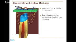
One thing that we haven't really talked about but which you'll see in the in the lab, and also like to just talk about it from from a physical perspective. If we now think about this particular experiment that we've got so we're going to look, let's suppose we've got some more body underneath this is one that was representing. This blue is a resistor up here and then we've got something out here, that's conductive and then even more conductive core and our goal is to try to find out what this guy looks like.

A

So we're going to do this experiment where we're going to put on an electrical current at the surface, so we're going to put a positive, electrode, negative electrode so now, we'd expect to see currents that are going to flow through there and those currents are going to get deviated because of the resistivity structure. Just as I was showing you last time with you know with the sphere, so we expect the currents both from here to there but I'm going to flow around one of the things.

A

That's very important here and it's kind of a physical principle. It's associated with this is that the electric yield, if I'm, trying to drive a.

A

Once I've got something like this and I'm trying to drive a current through here, then the principle that's always required is that the normal component of the current density must always be constant. So the result of that is that if I've got so remember, the current density is equal to a times Sigma or Sigma times the electric field. So if I've got something here of signal.

A

1/2 and now I've got an electric field. That's that's! Coming in here and I've got a current density. That's going to flow through, so I've got a current. That's that's going to be constant. On this side, I've got a j1 which is equal going to be 6 1 times 1. So, let's suppose I've got one here and a sigma and on this side here, I've got j2, which is equal to Sigma 2 P 2, so J 1 has to be equal to J 2 so that normal component current has to be the same.

A

So if J 1 is equal to sing 2, that means that Sigma 1 e 1 is equal to Sigma 2 e 2, ok, but these guys are different if Sigma 1 is not equal to Sigma 2. That means that II 1 is not equal to T. In other words, the electric field is discontinuous.

A

The only way, if you remember from maybe first-year physics, if you have a layer and there's there's a positive charge on that layer, then the electric field goes out like this from the positive charge here and electric field goes out like that from positive charge, so positive charge, every the fields can emanate outwards, and that means that there's a difference between the fields from one side to the other, and that depends upon whatever this charge density is so.

A

The fact that we've got different electric fields here means that there must be charges that are built up, and on this case here we have negative charges on this side. The positive charges on this side and the establishment of those charges then gives you that connection with what is actually going to be measured at the surface, because we'd remember, if you ever had a positive charge Q, then there was a voltage that was associated with that which was 1 over 4 PI epsilon, naught cube upon R, so I forgot if I've got any charge.

A

That gives me an electric potential okay, so the procedure is that we establish we cut a current into the ground, the current sort of flows through at regions where there's a change in the conductivity. There has to be some charges that are built up those charges, each give rise to an electric potential that that we can measure and it's those that net result. That gives rise to that number that we see from the DC resistivity survey.

A

So we put this current in here. It flows through there's charges that are built up wherever the conductivity is changing, and then because we've got Coulomb's law, which tells us that the voltage depends upon which other elementary charges divided by the distance with a scale factor. We just sum all of these guys up and that will tell us what the potential is at each of those places, and then we can measure the potential.

A

So that's the basic physics. Actually it's much simpler than the stuff that you saw previously with Maxwell's equations and induce currents, it all effectively kind of comes down to charges that are built up inside the earth.

A

Okay, so what do we need to do some important elements we need to somehow.

A

Figure out what we're going to try to find okay, so we're trying to find an object that looks like this and we got to put our currents sort it into the ground in such a way that they're going to couple with the object.

A

So we need to have currents that are flowing through once I got those currents that sets up charges and then the voltage, so you imagine targeter, set up here and then now I have to measure with some kind of an instrument sort of what that voltage difference is so I'm going to try to position those electrodes so that I get a number. That's that's true.

A

Okay, so this I think we we saw we've just done in the app in the lab. This is the characteristic figure that you have your positive current here at negative current here. So the voltage from this positive Kirk comes out like that. Like that and then we'd measure some voltage difference between any of those two two parts, and then we can use that to calculate an apparent resistivity.

A

Something that I think is intuitive.

A

Suppose that I've got a layer, I've got a silver one here, yeah and now.

A

So the idea is that they want to put in you know some kind of a current through here that is, is going to recognize that you got a boundary under here. So maybe this is bedrock or just some other layer if you're at a situation like this, so basically the kind of the current sort of flow through like this and because you're the spacings between your current electrodes are perhaps much less than what we've got here.

A

You kind of get the idea that virtually all the current is going to flow in this upper region, which means that you're only going to be sensitive to what's going on here. So if you plotted the apparent conductivity or maybe here, I could've used resistivity.

A

If we do a measurement of an electric potential in here, then the apparent resistivity I'm going to get is basically just going to be due to this this guy here and so I'm going to look at some value here. So this is that's real one, and now, if I, let's suppose I keep that st. geometry, but I just make it progressively bigger. So I could start here's.

A

My a B mm and I'm going to think about this whole thing being compressed or gradually made bigger and bigger, and so I could put on a sort of a scale length here for for my survey and so I could plot scale like yeah when my scale length is actually much less than whatever this thickness is. It's called an H, so maybe that's each year when we're much less than that. My apparent resistivities are probably going to be pretty close to know what.

A

If, however, I make this thing really big, so if I plotted and wanted different scales so that effectively you might this layer thickness, looks like this and now my currents are this, this kind of size. Now you might get the idea well, this layer thickness here is so small that we're not really even seeing it. So it's basically all the currents are kind of flowing in here and that for scale lengths that are really big I'm, actually going to come up to something that's more like roll in between.

A

You might kind of think that that curve would look like this. So that's exactly what happens. I mean I, think you might have sort of got that just sort of feminine to add a new point, but if you actually carried out the numbers, you'd see that the same that same thing happens if you, if your sampling array is really small compared to the depth that you're interested in then you're just going to be sensitive to this. If it's arguable that I'm not sure that you see dummy.

A

A

When you look at the epic EPG, you'll be able see, so this is that kind of electrode spacing, and this is the apparent reasons given e and when you're really small, you start out with the upper layer to the bottom.

A

So, there's a whole host of ways that you can acquire data and you'll see different names for different types of surveys. A lot of these have a degree of symmetry. That's that's attached to them. This one, for instance, has got four electrodes and they're each the same distance apart, so I've got a current electrode and then some distance, a I've, got a potential electrode.

A

B and all of these are a distance a apart and that's just a configuration that people have taken data for years, so you're going to see that name, it's called a winner array.

A

The other kind of thing array that you'll see is something called a Schlumberger array which is kind of like this, except these electrodes. Here the M&E and.

A

That distance, here at between m and n, is actually much less than the arc.

A

So it's it's still an electrode array. That's symmetrical about some some midpoint, but for whatever reason you know they chose to have these two things actually very close together. So that's a winner and an lumbering and you'll see these a lot.

A

Sometimes environmental serve will tend to emphasize these, and the way they operate is in something called a sounding mode and that's basically to take a point.

A

So you pick a point here and then you start with your rate compressed and then you just gradually get bigger and bigger and bigger and bigger and.

A

Effectively, what you're doing is kind of expanding around some central point, and then you can plot an apparent reason stivity as a function of your scale, length of your array, and then you get some kind of a curve.

A

Maybe that looks like this, and the idea with this sounding is that you're, your kind of central point of your array is this right here, just gradually making it bigger and bigger, and as we do, then the currents go farther and you're somehow deeper, as you increase size, you're looking deeper, but you're kind of thinking of being rich.

A

So that's the first thing is you know, and if things were really one-dimensional, then that's really all you need where you just sit someplace and just expand them, but in many cases what we're looking for is something that's varying laterally. So suppose we've got some some object in here then, as you as you sort of move over here. What you're trying to do is to try to find this this guy, and so you might try the following thing: it's like! Okay, let's fix an electrode array. Suppose I took something.

A

A

I'll, take us out, I'll put it here, I'll get a number for here and then I'd look to see what the apparent resistivities were as I go over here and the apparent resistivities it might be up here and then, as I go over. It drops down- and it comes like this, so this is now distance. Oh this way and I'm simply just taking my array and moving that would be called a profile.

A

So I'm I've got my array and I'm moving it over across like this yeah and if there's some parts that are particularly exact literally just I might see some. So that's good for lateral changes.

A

But there might be cases where you kind of want to do both, because, if I fix mild, if I fix my array, whose my current use my potentials, there's there's kind of a depth of investigation. That's associated with this particular array. There's a there's, there's a sensitivity down that at some depth and if the object that I'm looking for happens to be in there I'm that's great. But if my object is down here or if it's small or not there, then it might be. The battery is not actually a really good one to use.

A

So in that case, what I'd like to do is to hedge my bets a little bit and say well: I'm gonna go over with one type of array in a profiling zone and then I'm gonna take a different I'm going to take a different array may be suppressed or wider, and and also pull it over. So that would combine and the two aspects of the sounding and the throw flop.

A

And if you'd like to see how people are acquiring data these days, that's basically what they're, what what they're doing so first of all to talk about the profiling get a whole bunch of different types of electrodes. So this one is called a pole pole.

A

And, of course, you always need to have four electrodes, but if I've got an area of interest, so let's close, my area of interest is like this and I take my eighth electrode and then I run like so here's my generator and then I put my B electrode way and I can gone someplace and then, if I had my M electrode for my potential and I put my an electrode way in heck and gone, then really.

A

The only thing that I'm kind of considering about is basically just a current pole, electrode and a pole potential electrode so that kids best a pole, pole. Okay, you also have a pole dipole. In fact this is the one that is is very often used in in Merrell exploration, so would take run the alias or this other current electrode of heck and gone, and instead of yes/no for potential electrodes, we've got an and I sometimes use dipole dipole. This is actually more heavily used in kind of environmental types of surveys.

A

The reason for that is for the pole, pole, you evaced amount of penetration. You have the smallest resolution for the dipole dipole. You simply the shallowest amount of depth information, but the highest resolution, and these guys are.

A

So those would be the profiling modes and because, as I just said, what we'd often want to do is to do both of these together to both profiling and sounding then what we're going to do is decide on a rate, so it could be a pole pole. It could be both I pole whatever and then we're going to move it along. So that's the profiling and they were going to expand things, make it bigger. So that's the sound, so we've put them all together and we end up with something that looks like this.

A

This is kind of how we do it. We have a current source, and generally we take the the the current and instead of just turning it on and leaving us do the photo. We turn it on and we leave it for a while. Then we turn it off, and so what wow this is happening. My my voltage here with the curtains office is gone, so this is I. This is time my voltage down here.

A

Is nothing when there's no current? No current goes on now. I get some voltage leave that on and then at some point, I'm going to turn the card off goes down like this, so my voltage signal looks like this and then I'm gonna need this loss for a while and then I'm gonna turn it back on, but in the opposite, polarity and then be like this. We'll talk a little bit more about exactly why we do this.

A

This is because of this IP experiment that I talked about, but this would be sort of the nature of the current that you put in, and the voltage then you'd expect would so for each of these voltages that you get. We could compute that to some apparent resistivity, so we've got but the voltage we got the currents. We know what all the geometry is. So that gives us an apparent reason stated when we're going out and do an experiment.

A

We've got sort of the start position of our survey and position, we're looking for it for something in here. We've got whatever. Maybe it's a pole, dipole or something experiment and we're going to move this along and we're also going to expand it. So that means that we need to have some way of at least plotting up the data and the way the data can be plotted is something called a pseudo section.

A

And I want to explain how that is so, here's here's our system, so we've got currents potentials, so we can measure that potential Delta B. We know what the current is. We know what the geometry is. That gives us an apparent resistivity. Okay, we're not going to plot that somehow, so we can imagine that we're going to make a plotting plane.

A

Let's suppose, we've got a dipole dipole survey as the way we choose to do this is that we will draw a diagonal line, 45 degrees from the current dipole and at 45 degrees from the potential dipole and have where they intersect. That's actually, where I'm going to plot the data, so I'm going to find an apparent reason, stivity value in applying time right there.

A

A

Move this away, what happens to the plotting value? Well, we still have we're still along this 45-degree angle, we're still along this one, but now they are going to join here. So the farther these guys move away the deeper in the plotting playing the numbers as plot.

A

So you kind of can see how this is going to go right, but the farther this moves away, I'm going to get to be able to plot this date in a way that at least as I go down here, I'm going to be thinking somehow I'm going down in depth. So this is not going to be a true death. It's just going to be kind of representative, but it's sort of hope that maybe things will give you some inkling of.

A

What's there geologically, or at least it's a way of plotting, so now we continue to do that.

A

So you gradually get down okay, so that would that would be that. So now we can imagine here's here's our whole survey, so you can see what's happening here. So we continue to move the a the current electrodes and then this guy potential electrodes continues to move out and each time we sort of plot them the values we got the parrot resistivities and then we can contour them up. So the reds are regions of low resistivity and the moves are regions of high resistivity. So let's just do that again.

A

Okay, so you can see what's happened here, this has moved over one unit. This is actually moved over quite a few 45-degree angles over here and.

A

A

So you can see we're gradually building up our plot.

A

Right so now all of these are just values and then once we get to the end of the plot.

A

Contour it up so for people I mean people will actually seen a pseudo section, one just one one so for anybody, who's done a dcpip experiment, and this is generally at least traditionally the way the data are plotted. At least that's in surveys in which the data are collected along a line. So your currents and potential electrode.

A

That was a part of the data. What I want to emphasize is that there, even even when we talked about that sort of sphere right, and so we got a current that comes in here, so we got currents that are kind of going like this and I said. Well, you know that's going to give us two charges up here and maybe other charges down here.

A

Each of those contributes to some potential up here and at the end of the day, we're going to take that number and we're gonna get one apparent: resistivity 120 ohm meters and we're gonna plot that at some particular point.

A

That plot does not specify that at this particular depth at this particular location, it's 120, ohm meters, it's it's just a plot. The number that you get really depends upon everything that's happening in the volume. In fact, that's one of the things that characterizes a lot of geophysical data. We get a number out, but we need the understanding. That number means that you have to understand where currents or charges are everywhere in the subsurface. So it's just a number.

A

Similarly, when you put all that together, this image of the data that you have here is just the picture. That picture might tell you something geologically in this case. It does actually so here's a case whether you've got a buried prism. Okay. So this is a conductive prism, resist a background, this dipole-dipole experiment over top of here we actually get this pseudo section. That looks like this well, this doesn't look like that, but you know it's got some things that are so traded that, like the high.

A

High conductivity or low resistivity, it's kind of centered right around here, which is more or less where the center of the yes and you know for a trained eye. Somebody's had a little bit of experience and you're going to spot a dribble. You look at this and say: oh I'm, gonna just spot something right in here, I! Think there's something right under me. In which case have you done that you'd been quite successful.

A

The thing I want to emphasize is that when you just take is background, geology and you start just start putting little bits of junk in sort of make some plays- and you know good graphics or whatever it's just your little bit of crud up top and then you do the same experiment.

A

You now get a d-series stivity suit, a section that looks like this. So now this is completely uninterpretable. You can't you simply can't do anything with this. It's just stuff that's happening because of all of that ground. So you've got all this work. You collected the data. You've got a picture of the Gator, but doesn't tell you anything and again. Remember that you know each point that you actually have here is just a reflection of everything that is existing in that whole region.

A

So here is a case now where you absolutely have no choice, but you got to do something, that's more sophisticated. So now you actually have to invert these data, so we don't, unfortunately, have very much time to talk about this, but give you a quick. So basically, what we're doing we've got. Other measurements got some data, and the purpose of the inversion is that we want to somehow go back and try to find what that earth model is. So in this case we want to find that electrical conductivity.

A

In order to do that, we actually have to do a whole workflow. Everything from you know collecting the data understanding.

A

What the data are, our certainties that have to discretize the earth divide the whole bunch of little blocks and then we're going to have to adjust the values of those blocks so that we actually go ahead and fit the fit to data, so the process is involved but doable, and if we go ahead and not take a look at this example, our resistivity, this is our suit of section, doesn't mean anything, but if we take that- and we put it into an inversion- we get not something that looks like this, so it's actually but a lot of really good features right.

A

So here's here is our block that we're interested in it doesn't have sharp boundaries. It's not smooth, but that's, okay, and you can hurl'd here you get this, and the other thing is that all this junk that was sitting out here with actually recovered it. So the inversion has kind of recovered the locations of that of those other pieces of conductivity.

A

So we can do that and now that processing not only needs to be done, but is standardly done. In most cases the the earth I showed you there was was sort of 2d examples in real cases. Now you have to contend with the fact that the earth is is 3d so that all kinds of topography done the objects under the crown might be sheet served dikes or something like this, and so you've actually got to do this in 3d.

A

So I want to show you one one example, so this was stuff that was done from Australia a number of years ago. So the area this was a mineral deposit. So this is about two and a half kilometers on this axis here, and this is about four kilometers here and when we're looking at our ten lines of data.

A

So each of these lines of data there was a pole, dipole experiment. So one end of the current wire was run a couple of kilometers off the end here, and so we had a pole and then we measure the electric potentials along here and what you're seeing here, the pseudo sections that I was just talking about on each of these lines, with the following geometry, which is a dipole pole, which means that the electric potentials were on this side and the current source was on here.

A

Redis indicates low, resistivity, high conductivity, and so you can see that oh there's there's some stuff happening here as I go through these different lines. There's there's some red red things here right. So it's telling you something, but that doesn't give you a geologic picture. So if you excited the earth differently- and we could do that simply by reversing the whole situation, I could put the current electrode on here.

A

So now, I'm igniting the earth differently because my turrets are coming in from this direction and again these center sections now you've seen pseudo sections changed a lot. There's still something kind of red over on this side and there's things that are more blue, but that doesn't it doesn't give you a geologic understanding of what's going on so we've got all of these pictures and we need to somehow combine them to get a single there's. Only one earth bottle up there.

A

So what we want to do somehow combine all those images and see if we can find something a geologic. So we do that so now. What we do is we take those as data and then we take this mathematical cube for the model.

A

We take an earth model divide it up into a whole bunch of cells on its thousands or millions of cells, and then we adjust the values of these cells through the inversion so that we get all of these data at the same time, finding something that's kind of reasonably smooth, and we do that. We get a cube. So what I'm going to show you now is it's a three-dimensional cube that has been color-coded, so the red means that numbers are. The cell values are really conductive oops.

A

And what we're going to do now is slice through this guy and a couple different directions so now we're slicing from kind of the south to the north and then we're going to kind of come back again and you can see as we do that there's. The prominent thing is this red block up here.

A

And now we're going to slice from the top down and you can see again there's this big red right here. So that's that's got to be a big conductor. That's going to come up.

A

And now what's happening is the cube is spinning, but as it spins the ISO surface, at which things become transparent, get progressively changed so that at the end, we're only going to see the most conductive parts of that whole 3d model.

A

And in the end, it looks like this, so here is your three-dimensional image of the geology that was underground that actually produced those data. At least this is the biggest element here. So this element is actually a black shale unit. It's very conductive and it's by far the most dominant dominant component for establishing, but the signal is for that that DC resistivity surveys. So that's the good news we've taken all of those pseudo sections and we've manipulated them into getting something. That's geologic.

A

uh The bad news in this case is that what they were actually looking for. It was a mineral deposit, and this guy is not marelize he's not anything. That's particularly useful, however, the same experiment that I just talked about where we had her. It goes in like this. So here was my turn.

A

There's a companion experiment, while it's done at the same time in which, instead of just measuring this number here and getting the apparent resistivities, you actually look at what happens after the current turns off. So when this current turns off, it turns out that there's going to be a decay voltage here that decay voltage is indicative of the fact that the earth can actually charge up. It has some charge ability, and that gives rise to another datum, which is called the IP datum or induced polarization data.

A

So what I'm going to do next time, I'm going to pick it up from from here we're going to talk about this part of the curve that comes down, how it is, what causes it and how we can extract information about the Earth from it, and this guy turns out to be one of the most I think important aspects of mineral exploration. That's probably cropped up in the last. You know 30 or 40 years. Certainly anybody who has got a pork redeposit that would definitely be associated with them anyway.

A

So that's coral pick it up on Wednesday thanks.