►
From YouTube: EOSC 350 Lecture 7: Magnetics 5. Doug Oldenburg
Description
September 23, 2016. Fifth lecture on magnetics in geophysics: applications an interpreting data.
Slides are available at:
https://github.com/ubcgif/eosc350website/raw/master/assets/2_Magnetics/3_Magnetics.pdf
The Jupyter Notebook demonstrated is available through binders: http://mybinder.org/repo/ubcgif/gpgLabs/notebooks/Mag/InducedMag2D.ipynb and on github: https://github.com/ubcgif/gpgLabs/blob/master/Mag/InducedMag2D.ipynb
A
Okay,
so
this
is
ready,
30
from
which
we're
all
grateful.
Second
thing:
this
is
the
last
lecture
I
have
scheduled
for
my
headaches,
so
I
have
a
married
number
of
things
to
get
through
it,
I'm
going
to
be
flipping
through
slides,
pretty
quickly,
because
it's
a
lot
of
moving
to
just
step,
go
ahead
and
look
at
yourself
there's
one
or
two
things
that
I
think
are
important.
A
It'll
take
a
little
bit
of
time
to
go
through
I'm
going
to
concentrate
on
those,
but
in
particular
they
have
to
deal
with
your
TBL,
I'm
trying
to
understand
how
we
can
look
at
the
signatures
from
from
a
very
pipe.
So
that's
that's
the
technical
thing
of
significance
and
the
rest
of
us
I
want
to
just
go
to
quickly.
A
So
from
the
point
of
view
of
data
processing
is
really
only
two
things
that
are
important:
one
is
removing
the
Earth's
magnetic
field
and
the
time
the
time
variations
and
that
for
that
we
have
established
a
base
station.
So
you
did
that
at
the
beach
and
the
other
is
removing
regional
trends.
So
I'm
going
to
just
flip
through
these
guys
and
then
we'll
get
on
to
read
movement
so
time
variations
externally,
internally,
lots
of
stuff
happening
from
the
Sun
local
things
with
you
know,
generators
and
various
kinds
of
infrastructure
noise.
A
But
the
main
thing
is
what's
happening:
you'll
from
the
from
the
solar
system
time
variations
can
anything
from
minutes
to
hours
to
today's
anything
from
hundreds
of
nano
teslas
to
thousands
of
nano
teslas.
So
we
have
got
a
lot
of
variations
and
what
we
do
is
we
generate
a
base
station
measure,
the
magnetic
field
at
the
base
station
as
a
function
of
time
synchronized
with
our
receiver,
that
we're
collecting
the
data
with
and
then
perform
the
correction
by
subtraction.
A
So
that
was
a
time
Barry
we've
done
that
before,
but
the
other
dip
aspect
of
processing
is
that
we're
measuring
data
in
the
presence
of
the
Earth's
field
as
well.
As
you
know,
we're
interested
in
something
of
a
scale
size
like
this,
and
there
might
be
some
big
object
out
over
here.
That's
just
adding
a
big
signal
to
this,
and
we
really
we
really
don't
care
about
this
guy,
we're
not
trying
to
find
him.
A
A
So
that's
that's
good
of
that
background
field,
and
here
is
our
anomalous
field
that
we
want,
and
we
need
to
separate
these
two
things:
it's
not
a
trivial
matter,
but
we're
somehow
going
to
try
to
estimate
what
this
background
is
and
then
we're
going
to
subtract
it
from
the
observations
and
then
we're
going
to
be
left
up
with
the
residual
field.
That
looks
like
this
and
then
we're
going
to
say
off.
That's
our
anomalous
field
and
I'm
going
to
try
to
interpret
that.
A
Ok,
what
is
that
background
field,
and
that
takes
that
if
we
can
do
something
or
numerical,
but
there's
also
some
subjectivity?
That's
what
simple,
and
in
fact
you
could
see
that
if
I
didn't
have
this
dashed
line
here
and
if
I
asked
everybody
to
draw,
you
know
some
kind
of
a
background
field.
You
can
see
that
some
people
might
draw
something
that
looks
like
this.
A
You
also
might
go
up
into
here
or
some
other
direction
so
separating
that,
drawing
that
regional
field
is
not
a
trivial
operation
and
to
emphasize
this,
this
is
an
Aryan
British
Columbia.
It
has
the
Mount
Milligan
deposit,
which
I've
mentioned
a
couple
times,
but
it
is
one
of
the
most
recent
minds
to
go
into
production,
Crocker
or
three
deposit.
A
This
is
a
magnetic
map.
Red
is
high.
Magnetics
blue
is
low,
so
this
is
65,000
nano
teslas.
This
is
57,000.
So
there's
you
know:
8000
nano
teslas
difference
between
high
flow.
What
you're
seeing
up
here
this
leading
up
here
if
it's
mount
Milligan
right?
This
is
a
mountain
lot
of
magnetic
material
in
here,
and
the
Magnetic
map
is
really
you
know
completely
overwhelmed
by
just
this
great
big
high
and
gradually
getting
to
get
into
a
local
turns
out.
That's
not
what
is
of
interest.
What's
of
interest.
A
Is
this
region
in
here
in
this
box,
and
if
you
look
at
just
that
region,
you
know
you
can
see
it
kind
of
dominated
by
this.
This
red
card
in
here,
which
is
all
part
of
the
mouth.
So
that's
not
that's
not
what
we're
trying
to
get
here
we're
trying
to
get
magnetic
signature
in
this
region.
That
might
just
be
reflective
of
this
metal
deposits
underneath.
So
what
we
have
to
do
is
to
take
this
large-scale
map.
A
A
It's
the
result
of
having
taken
that
initial
data,
estimating
a
background,
subtracting
it,
and
now
you
can
see
what
we
got.
So
we
got
a
high
magnetic
anomaly
here
and
high
magnetic
normally
there
and
now
we
could
take
these
data,
go
ahead
and
invert
them
and
come
up
with
something
that
it
is
more
useful.
A
So
that's
F,
that's
sort
of
the
basic
scenario.
We're
not
going
to
go
into
details
about
I
would
do
that,
but
basically
for
every
magnetic
survey
that
you're
going
to
do
you're
going
to
get
rid
of
these
time
variations
and
then
you're
also
going
to
try
to
somehow
get
rid
of
some
background
so
that
in
the
end,
you're
left
with
an
area
over
which
you've
taken
data-
and
it's
just
all
reflective
of
some
local
objects
underneath
here,
and
so
you
can
think
about
this
as
the
anomalous
field
due
to
the
size.
A
Ok,
so
now
I
just
want
to
present
a
couple
of
examples
of
magnetic
data
and
then
we're
kind
of
going
to
go
through
how
we
might
might
think
about
this.
So
this
we
already
talked
about
this
guy
we've
seen
before,
but
now
you
recognize
that
each
of
these
yo
is
a
pattern
due
to
a
magnetic
dipole
that
is
situated
in
different
directions
and
that
you
now
also
understand
that
these
signatures
are
coming
in
a
large
part
from
remnant.
Magnetization.
A
A
The
easiest
thing
to
really
interpret
okay
is
the
following
situation.
Where
I've
got
you
know,
some
kind
of
object
is
sitting
here.
A
magnetic
field
is
coming
in
like
this,
and
now
I've
got
a
novelist
field
like
this
and
if
I
plotted
it
out,
I
would
have.
You
know
anomaly
that
looks
like
this,
so
that
if
I
looked
at
the
high
point
of
the
anomaly,
Doug
straight
down,
I'd
see
it.
So
that's
what's
happening
here.
A
A
A
The
thing
that
you
can
do
with
potential
fields
is
the
following:
I
could
take
any
of
these
data
sets
that
are
here
and
I
could
take
their
Fourier
transform
if
I
said,
Fourier
transform
how
many
people
would
know
what
it
is
right,
hey.
So
we
will
do
some
processing,
which
just
happens
before
a
transform,
but
we're
not
going
to
go
there.
So
we're
going
to
take
these
data
put
them
through.
A
A
Oh,
the
object
is
directly
underneath
you
because
for
this
guy
here
you
know
the
object
is
not
under
the
high
spot
and
for
this
one
here,
it's
not
even
original
high
spots,
a
low
spot,
so
that
reduction
to
pole
turns
out
to
be
a
really
really
useful
processing
step
and
that's
what
this
whole
system
does
so
sometimes
you'll
call
it.
Instead
of
four
you
transform
they'll
call
it
hurry
filtering
or
whatever,
but
it's
just
a
process,
so
you
don't
eat.
You
know
how
that
process
works.
A
Good,
so
that's
that's
the
first
thing
and
that's
an
important
thing,
because
then
that
helps
you
see,
you'll
make
a
better
relationship
between
the
image
that
you're
seeing
and
any
objects
in
it.
The
next
thing
I
want
to
talk
about
is
how
to
interpret
simple
bodies
or
how
to
interpret
the
magnetization
of
bodies
that
have
a
simple
shapes
and
a
uniformly
magnetized
and
a
particular.
A
A
So
so
far
we've
always
talked
about
you
dipoles
right,
but
you
know
a
dipole
has
got
you
look
kind
of
like
it.
We
can
think
of
it
as
a
charge.
One
end
a
negative
charge
of
one
man
and
a
positive
charge
at
another
end,
and
that
actually
turns
out
to
be
useful
in
practice
and
just
sort
of
how
to
think
about
things.
I
want
to
take
you
through
them.
A
A
So
if
we
got
half
a
dozen
parameters,
then
we
can
attempt
to
doing
something
it's
a
little
bit
more
sophisticated
and
that
is
to
try
to
match
the
observed
data
that
we
obtained
with
something
that's
predicted
by.
Let's
hypothesizing,
you
know
a
magnet,
that's
in
this
direction
and
see
what
the
the
data
would
be.
If
it
doesn't
fit
quite
well
enough,
we
could
change
the
orientation
strength,
the
location,
and
so
that's
the
idea
that
we've
got
an
object.
It
gets
rise
to
something
that
looks
like
this.
A
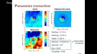
Now
we
want
to
do
some
little
bit
more
sophisticated
modeling
to
try
to
find
the
location
of
the
magnets
in
its
orientation
besides
such
that,
let
me
down,
went
back
and
generate
the
data
from
that
that
we'd
get
what
was
it
was
quiz
matching,
so
here's
here's
an
example
of
that
we
have
some
data.
Look
like
that.
We
have
an
algorithm
that
tries
to
find
parameters
of
that
magnet,
and
this
is
the
you
know
the
predicted
data.
A
If
we
do
the
difference
between
our
observed
and
predicted
data,
we
end
up
with
something
that
looks
like
this
looks
a
little
bit
choppy,
but
the
the
size
of
these
numbers
is
actually
pretty
small
compared
to
the
data,
so
we're
actually
doing
not
such
a
bad
job.
And
then
the
thing
that
we
obtained
is
the
depth
of
the
ordinate
side,
of
where
it
is,
if
XY,
how
big
it
is,
what
its
moment
is
and
what
its
what
its
angles
are.
So
that
actually
turns
out
to
be
very
important.
A
So
here's
now
where
I
was
just
a
second
ago,
I
want
to
bring
in
a
solid
concept,
so
we're
going
to
introduce
a
magnetic
charge,
Q,
okay,
and
if
we
have
a
magnetic
charge,
then
if
we
have
a
positive
charge,
it
radiates
the
fields
outward
that
look
like
this.
So
there's
a
positive
charge
Q,
and
we
actually
refer
to
this
as
a
monopole.
A
They
don't
exist
practice,
but
we
didn't
think
about
this,
and
that
would
be
a
positive
Church
and
there's
actually
a
formula
for
how
that
magnetic
field
buries.
It
depends
upon
the
strength
of
the
charge
and
it
depends
as
one
over
R
squared.
So
as
I
go
with
that's
just
like
a
leer.
It's
like
a
mass
particle
as
I
go
away
from
here.
The
field
varies
as
one
over
R
square
and
the
value
that
feel
goes
radially
out.
That's
where
the
r
hat
is.
A
A
A
Then
the
magnetic
moment,
like
the
strength
of
this
magnet,
is
actually
given
by
the
product
of
that
charge
and
the
distance
of
separation
/
binding
are
so.
That
is
the
magnetic
moment
of
that.
That
dipole
and
the
magnetic
field
from
that
dipole
is
something
that
looks
like
this.
So
it
kind
of
goes
goes
out
from
the
positive
pole.
Swings
around
goes
into
the
negative
pole,
so
it's
thing
that
you've
been
drawing
for
the
last
week
and
a
half
right
these
these
dipole
lines,
but
there
is
a
mathematical
expression
that
actually
call
or
qualifies
for
you.
A
What
the
magnetic
field
is
adding
a
point
out
here
and
that's
given
by
this
quantity
here
that
B
is
related
to
the
strengths
of
the
magnet
over
r
cubed.
Remember
we
were
talking
about
how
how
the
field
decays
away
from
something
for
one
over
r
cubed
and
then
we've
got
both
of
our
half
and
an
e
to
have
sign
convention
is
that
if
the
magnetic
moment
is
plugging
in
this
direction,
then
there's,
if
you're
sitting
at
some
particular
point
here
and
there's
an
angle
between
you
and
this,
this
axis
of
dipole.
A
That
has
that's
the
theta
angle,
and
so
that
is
the
angular
goes
in
here
and
then
there's
your
certain
distance
out.
So
that
gives
you
how
far
out
you
are
your
radius
vector?
The
magnetic
field
has
got
two
components.
It's
at
any
particular
point.
It's
got
a
component
out.
This
way
add
a
component
in
this
week,
so
it's
got
a
theta
component
and
an
hour
component
and
that's
given
by
this
formula
here
site.
A
So
I
guess
says
you,
as
you
know,
so
these
things
as
I
said
always
are
in
in
pairs,
and
how
do
we
actually
know
how
these
things
are
in
pairs?
What
was
the
first
experiment
that
anybody
ever
did
to
try
to
dissect
these
things?
Hey
people
have
always
wanted.
Okay
can
I
can
I
actually
find
a
magnetic
pole
right,
so
here
we've
got.
It
died
for
me,
so
I'm
going
to
find
a
magnetic
pole.
What
would
be
the
first
thing
you
think
about
doing
cut
it
in
half
right,
so
you
could
take
this.
A
13
bucks,
oh
God,
thank
used
to
be
I'm
not
used
to
get
cell
phone
right.
I
know
what
actually
happens
if
I
not
take
these
two
things,
I
kept
coming
together
right,
so
I
must
have
these
two
things
are
equal,
so
it
doesnt
sit
so
I
haven't
in
fact
nice
rich
part,
I
just
broke
it
in
half
and
I've
got
to
30.
To
get
so
I
did
mine.
Do
the
next
one
I?
Don't
you
go.
A
You
got
two
poles
or
you
have
two
dipoles
to
double
AA
state
mom.
So
now
you
can
give
it
to
the
Genesis.
Next
we
go.
We
will
just
see
how
far
we
can
go.
Okay,
Oh
sacrifice
him
a
poor
man
all
right.
Okay,
so
we
can't
find
a
pole
right,
so
we're
only
getting
two
dipoles
and
the
dipole
is
actually
going
to
you'll
have
an
expression
that
looks
like.
A
So
why
why
is
this
useful?
It's
useful
in
the
following
sense:
if
I
take,
if
I
take
any
piece
of
material
okay,
so
it's
got
a
lot
of
your
magnetic
particles.
You
know
I
can
actually
think
about
these
as
being
your
little
magnets
inside
right,
so
that
because
everything
gets
magnetized,
so
I
could
think
about
dividing
this
video
I'll.
Do
it
by
now
yeah.
A
A
But
now,
if
I
think
about
it
so
what's
happening
up
here,
I
have
a
negative
charge
up
here
on
that
end
of
the
arrow,
and
this
end
here,
I've
got
a
positive
right
and
in
here
I've
got
a
negative
here.
I've
got
a
pause
if
you're
going
to
negative
you're
gonna
pause,
you're
gonna
function
that
does
death
time.
You
know
effectively
these
guys
here
kind
of
cancel
out
so
I'm
sitting
up
here.
So
I
got
these
guys
counts.
We
know
these
guys
can
still
close,
and
that
was
positive
negative.
A
So
those
cancel
out-
and
the
only
thing
I'm
left
with-
is
some
kind
of
negative
charge
up
here
and
a
positive
charge
stuff.
So
it's
an
equivalent
way
of
thinking
about
it,
even
though
it
truly
everything
is
magnetized
in
here,
but
another
way
of
thinking
about
it
is
that
kill
all
these
internal
guys
are
kind
of
cancelling
out
and
really
the
only
thing
I'm
left
with
is
sort
of
like
a
neck
magnetic
charge,
negative
charge
of
pot
and
a
net
positive
charge
as
the
water.
A
Well,
if
that
is
actually
happened,
and
we
already
saw
what
the
magnetic
field
was
from
a
single
charge
right
then
all
I'd
have
to
do
is
just
you
know.
If
I'm
sitting
up
here,
I
just
have
to
add
up.
What's
the
effect
of
all
these
negative
charges
and
I
bought
the
fields
due
to
the
top
surface,
I
can
do
the
same
from
the
bottom,
but
remember
everything
falls
off
as
one
over
R
cube.
If
this
thing
was
actually
far
enough
down,
I'm
just
left
with
something-
that's
really
close
to
me.
A
A
A
A
The
magnetization
and
the
normal
vector
in
this
particular
case
up
here
I
grew
a
a
negative
sign,
but
if
I,
if
I
thought
about
it
is
m
dot
and
hat
so
H
naught
is
like
this.
So
the
magnetization
is
this
way
right
and
an
hat
is
the
outward
normal,
so
n
hat
as
if
any
for
any
object
is
always
the
outward
normal,
so
m
dot
and
is
minus,
and
hence
that's
also
another
way
of
thinking
about
what
what
happens
up
here,
that
we're
going
to
get
a
negative
charge
when
we
have
objects
like
this.
A
So
let's
suppose
I
still
have
a
cylinder.
Okay,
so
go
back
one.
So
if
I
come
back
here,
if
I
just
have
a
cylinder,
I've
got
a
magnetic
field.
That's
coming
down
this
way,
then
n
half
is
out
here.
So
that's
negative
at
the
bottom
and
hats
out,
that's
in
the
same
direction
as
H
naught.
So
it's
positive,
so
I
get
a
positive
charge
here
at
a
negative
charge
here
and
what
do
I
get
on
side?
A
Anybody
I
get
0,
because
an
hat
is
out.
This
way
and
m
is
down
this
way
there
at
90
degrees,
cosine,
theta
DZ.
So
the
great
thing
about
this
concept
is
that
I
can
take
something
that's
pretty
complicated.
I
can
take
you
know
a
big
cylinder
chunk
it
in
a
field
get
if
it
gets
magnetized
uniformly
that
actually
I
can
represent
that
final
magnetic
field.
A
Just
in
terms
of
you
know
a
few
charges
on
this
upper
surface
and
this
lower
surface,
and
as
I
said,
if
that
lower
surface
goes
to
something
that's
really
great
a
great
depth,
then
you
don't
see
it
up
in
here,
and
that
is
what
you're
going
to
use
on
monday.
When
you
do
your
team
based
learning
in
general,
if
I've
got
something
else,
if
I've
got
a
magnetic
field,
that's
coming
in
this
way.
I.
You
know
then
I'm
going
to
have
you
know
some
negative
charges
here.
A
Some
positive
charges
here,
the
nerd
okay
I-
can
still
figure
that
out,
like
I,
just
calculating
em
dance,
not
a
big
deal,
so
I
just
calculate
that
out
and
then
for
each
for
each
charge
right.
So
whenever
we
got,
you
know
some
kind
of
a
charge.
Remember
so
we
had
B
is
equal
to
MU,
naught
over
4
PI
R
squared
times
Q,
whatever
that
that
Q
was
so,
we
can
actually
calculate.
A
Okay,
so
this
is
this
leads
to
a
simplification.
We've
got
things
that
are
magnetized
uniformly.
We
could
think
about
those
as
dipoles,
and
that
gives
us
just
lines
of
charges,
strength
of
those
charges,
m,
dot
and
hat,
and
then,
if
you
take
a
any
kind
of
a
crazy
shape
in
here,
you
can
convert
that
just
to
the
charges
sum
up.
The
fields
from
each
charge
enter
your
problem.
A
So
on
Monday,
and
we
might
have
to
go
over
this
again
too,
okay,
hey
take
a
look
at
this
is
what's
going
to
happen,
is
so
it's
just
like
at
the
at
the
beach
right,
so
we
had
a
vertical
rod.
Okay,
it's
magnetized
in
uniform
direction.
We've
got
some
radius
vector
a
magnetization
gotta
charge
density,
so
the
total
charge
is
just
going
to
be.
A
A
The
fields
at
surface
just
become
a
little
bit
more
complicated.
In
the
end,
when
we
are
working
with
really
big
problems,
then
we're
just
going
to
have
a
whole
bunch
of
these
little
prisms
or
often
we
call
themselves
inside
here,
each
of
which
has
got
its
own
magnetization
and
which
produces
its
own
contribution
to
the
magnetic
field.
At
the
surface,.
A
So
yeah,
just
to
kind
of
quickly
quickly
go
through
this,
so
here
was
there's
now
a
magnetic
map
of
a
larger
region.
It's
it's
up
in
rhyme
with
so
this
is
this
region
of
high
magnetic
magnetism.
Here
is
what
we're
interested
in
and
there's
a
particular
region
here
to
exactly
where
this
image
came
from.
A
I've
shown
you
a
number
of
times
that
that
ragged
closet,
so
it's
just
coming
in
in
a
little
section
in
there
and
there's
been
a
background
field,
that's
been
taken
off
and
then
now
we're
going
to
use
that
principle
of
superposition
and
inversion
and
then
try
to
get
out
a
under
model
and
this
what
I've
got
sketched
out
here
is
essentially
the
same
kind
of
quantity
that
we
talked
about
with
the
parametric
inversion,
and
that
is
that
now
we
have,
we
have
a
big
model.
We've
got
lots
of
prisons
in
it
different
susceptibilities.
A
A
So,
let's
just
kind
of
rewind
back
to
where
we
started
a
couple
weeks
ago
for
the
general
use
of
geophysics.
Oh
we've
got
first
of
all
a
problem:
Simon
scientific
engineering,
whatever
we
figure
out
what
our
physical
property
as
we
go
through,
we
do
get
physics
decide
on.
Our
survey
is
of
data
processing
inversion.
A
Now
we
come
back
so
that's
in
terms
of
the
physical
property
distribution,
and
now
we
try
to
figure
out
okay.
How
is
that
actually
helping
address
the
problem?
Hey?
So
that's
always
the
sea,
and
we
have
a
framework
for
this,
and
we've
got
a
whole
bunch
of
examples
that
this
could
be
applied
to
and
I
want
to
just
flip
through
a
couple
of
these.
So
first
of
all
we're
just
going
to
see
what
inferences
we
can
make
just
from
the
data.
A
Here's
one
for
the
point
of
view
of
geology.
Is
it
terrible
can't
really
see,
but
you
know
there's
a
whole
bunch
trees
here
and
here's
there's
no
trees,
but
I.
Don't
think
you
can
see
that,
but
even
just
looking
at
you
know,
what's
you
know,
what's
growing
there,
you
can
see
right.
Ok,
this
is
really
different
from
what's,
and
so
you
mean
look
at
this.
You
got
charging
you
a
John
g-unit,
be
one
of
the
most
useful
things
for
magnetics
or
for
geophysical.
Surveys
is
magnetics,
it's
cheap!
It's
effective!
A
It's
used
on
a
regional
scale,
it's
used
on
local
target
scale,
it's
used
for
prospective
areas
and
that's
why
of
all
the
geophysical
data
you'll
see
it's
probably
going
to
be
magnetic,
since
it's
the
first
and
I
may
have
shown
you
this
before,
but
now
me
you
might
get
a
bit
of
different
insight
to
it.
Here
is
a
deal.
Here's
a
magnetic
map-
and
here
is
a
geology
map
to
wait
for
things
this
was
obtained
by
you
know
people
walking
around
looking
at
oak
crops.
A
This
is
paid
by
some
airplane,
that's
flying
over
with
Nick's
room,
and
you
immediately
look
at
those
two
things
and
you
see
oh
there's
a
lot
of
common
elements
in
particular
this
this
region
here,
so
wherever
you're
separating
units,
your
different
Rock
units,
as
long
as
they
have
a
different
susceptibility,
you
should
see
the
macaron
and
you
can
see
where
that's
happening
very
long,
so
finding
contacts
between
different
units-
that's
a
biggie
looking
through.
Maybe
these
are
intrusive
zones.
A
I
have
no
idea
what
what
these
guys
are,
but
I
mean
again
you
can
see
so
the
point
about
this
is
that
a
magnetic
image,
especially
when
tied
with
a
little
bit
of
geology
right.
So
if
you've
got
a
couple
of
ground-based
observations,
let's
say
here
and
here
denoting
that
you
know
this
is
rock
unit
1.
This
is
rock
unit
2.
Then
you
look
at
this
magnetic
map
and
you
have
a
first-order
extension
about
where
these
different
different
units
are,
and
that
might
be
just
hugely
valuable.
That
might
actually
impact
where
you
go.
A
Then
we've
got
faults
that
are
that
are
coming
through,
so
here
geologically
is
a
fault
that
has
has
been
mapped
and
very
often
on
a
fault.
There's
alteration:
that's
going
on
various
things
that
are
happening
to
change
magnetic
susceptibility
and
if
you
look
on
this
magnetic
map,
see
it's
just
extremely
clear
here
that
there's
something
happening
between
these
two
sides,
so
mapping
faults
mapping
Rock
units.
Those
are
important.
A
A
The
other
thing
that
you'll
see
about
magnetic
maps
is
that
they'd
already
put
the
magnetic
map
but
they'll.
Sometimes
you
processing
tune.
I
talked
about
one
process,
except
where
they
do
reduction
to
pull,
but
there's
other
things
that
that
you
can
do,
and
you
can
just
kind
of
regard
these
things
as
images
khatam
abyss.
That's
a
I
SAT
image.
This
is
a
topography,
and
this
is
surface
geology.
So
we
see
definitely
some
different
different
Rock
units
there,
and
so
we
can
look
at
a
number
of
things
here.
So
superimpose
the
black
lines
of
geology.
A
A
Looking
at
how
the
magnetic
field
changes
with
with
height
I
find
how
to
particular
well
I'm
at
a
particular
case,
I'm,
looking
to
see
how
it
changes
with
height,
how
quickly
it
falls
off
and
if
you've
got
if
you've
got
something
that's
very
near
surface
and
then
you
look
at
the
gradient,
you
find.
Oh,
it's
changing
very
rapidly.
If
you've
got
something,
that's
very
deeper,
then
it
doesn't
change
too
much
very
much.
So
it
gives
you
another
picture
and
every
picture,
especially
when
you
look
at
it.
You've
got
yes,
it's
got
some
correlation
to.
A
It's
got
some
texture.
It's
got,
you
can
see
things
happening
right,
so
all
of
those
are
somehow
being
related
to
to
geology
and
they
can
actually
help
kind
of
refine.
You
know
what
it
is.
You
think
you
might
be
looking
forward
where
to
find
more
of
it,
and
then
you
can
also
do
other
imaging
to.
This
is
looking
at
sort
of
angular
dispersion.
A
So
what
my
only
point
I
wanted
to
make
there
and
we're
not
time
to
talk
about
these
things,
but
you'll
see
magnetic
maps,
and
then
there
will
be
processing
this
done
on
some
of
the
processing
reduction
to
pole.
First
derivative
could
be
vertical.
Derivative
could
be
horizontal
derivative,
anything
so
look
down
the
scale
and
see
what
they're
doing
you're,
taking
a
derivative
you're
kind
of
looking
at
changes,
either
with
respect
to
elevation
or
horizontal.
Oh.
A
Okay,
I
mean
just
I
just
want
to
get
this
in
at
least
it
within
a
couple
of
minutes
cuz.
It's
such
a
it's
such
an
important
problem,
and
we
don't
see
it.
We
see
it's
something
to
an
extent
in
North
America,
but
it's
I
just
talking
a
whole
bunch
of
people
from
Europe
boat
over
the
last
weekend,
just
that
the
prevalence
of
scale
of
unexploded
ordnance
there
and
what
it's
causing
it
huge
but
I,
don't
know
that
you're,
aware
of
just
what
things
are
like
just
in
the
proving
grounds
in
the
United
States.
A
That's
like
this
is
San
Francisco
Bay
Area
right
for
toward
one
of
those
places
have
to
have
to
clean
it
up.
So
there's
a
central
lowered
babe
range
here
was
the
Fort
Ord.
So
it's
that
work
done
on
that
places
in
Hawaii.
Cahill
allow
its
sacred
ground
to
the
Native.
Hawaiians
needs
to
be
cleaned
up,
sometimes
there's
just
fragments.
Sometimes
it's
all
kinds
of
junk
and
I
showed
you
that
one
before
those
limestone
hills
in
Montana
and
the
way
they
used
to
do
it
was
these
sort
of
handheld
instruments.
A
Now
we're
doing
digital
work,
and
you
can
I
showed
you
some
examples
of
just
like
really
high
quality
work.
So
here's
something
it's
got
a
high
signal-to-noise
ratio
on,
but
sometimes
you
know
the
date
are
a
little
bit
happier
he's
a
little
bit
little
bit
worse
and
you
know
here's
something
else.
It's
you
know
things
that
are
kind
of
coming
and
but
you
can
still
see
it
and
then
here
you
get
places
where
okay,
what's
going
on
here,
there
is
something
very
new,
but
now
there's
so
much
noise.
A
So
you
get
things
are
not
always
textbook
examples
right,
there's
always
different
challenges
depending
upon
how
deeply
the
ordinance
is
buried
and
deaf
yeah
what
it
is
you're
looking
for
and
okay,
so
I
gotta
quit
rest
of
things
are
the
notes
it's
like,
maybe
maybe
monday.
I
might
have
a
good
fine
campus,
there's
about
10
more
minutes
here
of
just
how
geeky
do
a
little
few
examples.
We've
actually
done.
All
the
things
we
really
the
only
vaccine
or
just
a
couple
of
occupations
will
find
its
niche
sometime
in
the
thing.
A
A
Use
the
app
bills
build
something
that
looks
like
this
right
put
a
magnetic
field
on
it,
it's
pointing
vertically
down
and
go
through
the
computations
that
I
just
provided
you
on
the
board,
and
they
are
also
in
the
gpg
to
think
about
this
scenario
and
figure
out.
Okay,
what
is
the
charge
guessing?
What's
the
magnetic
charge
density
on
the
surface?
What's
the
total
charge,
ok
and
now
think
about
okay,
there's
that
total
charge
Q
if
I'm
going
to
do
a
magnetic
experiment
over
top
of
it.
A
This
is
what
I'm
going
to
get
and
then
importantly,
look
at
this
half
width
here
and
compare
that
with
the
death
of
burial
and
by
the
depth
of
burial.
We
actually
mean
the
death
between
the
sensor
height
and
where
the
top
of
this
guy
is.
So.
If
your
sensor
heights
melee
at
zero
and
this
guy,
is
that
three
meters,
then
that's
the
death
burial
and
then
you
should
get
that
this
half
width
is
kind
of
in
the
order
of
them.
A
So
this
is
going
to
be
the
real
ticket
thing
that
you're
going
to
do
for
the
TBL
kisser
there's
going
to
be
a
whole
bunch
of
examples
here
where
they've
gone
over
they've
looked
for
and
they'll
talk
about,
though
I'm
going
to
go
to
find
a
monopole
so
like
there
is
that
good,
we've
already
decided,
you
can't
find
a
monocle
right,
but
they're
they're
kind
of
an
equivalent
monopole,
because
they're
doing
something
like
this
and
effectively.
This
is
just
a
charge
here.
A
They
want
to
find
these
things,
and
you
know
how
hard
it
is
to
find
it
by
digging
right,
because
you
weren't
very
successful
so
you're
going
to
do
this
kid
physical
work
over
here,
you're
going
to
locate
where
the
pipe
is
and
with
the
half-wit
you're
going
to
get
approximately
the
death
the
burial
you
get
develop
so
work
through.
All
of
that,
it
will
consolidate
the
material
that
we
just
stopped
the
class.
It
will
really
make
the
TBL
cool
quickly
and
you'll
have
the
Star
Force
or
help.