►
From YouTube: EOSC 350 IP Lecture
Description
Induced polarization method in Geophysics. Lecture by Doug Oldenburg on November 23.
A
No
actually,
this
is
the
last
Mickey
lecture
because
look,
there
is
some
stuff
that
I
definitely
want
to
see
and
I
think
you
will
pick
up
line.
So
if
it's
actually
an
area
of
geophysical
research
that
I've
been
involved
with
quite
well,
and
it's
something
that
has
got
a
lot
of
importance
in
the
mining
industry,
especially
it's
becoming
more
important
in
water
resources
and
in
sort
of
environmental
contaminants.
A
It's
just
one
of
these
things
that
at
one
point,
people
didn't
even
recognize
that
there
was
a
signal
there
and
then
gradually,
as
instrumentation
got
better
and
people
look
a
bit
more
than
wait
a
minute,
there's
something
kind
of
happening
here.
Maybe
we
should
take
a
look
at
it.
Try
to
understand
you
know
what's
going
on
and
then
eventually
it
gets
to
the
point
where
this
is
actually
a
mainstream
and
it
hasn't
very
big
piece
of
information.
A
The
idea,
the
basic
idea
go
through
it
in
more
detail
is
that
the
earth
can
actually
act
a
bit
like
a
capacitor.
If
you
tried
to
drive
the
current
through
some
rocks,
then
they
build
up
charge
and
they
act
like
a
capacitor,
and
when
you
take
that
driving
current
off,
then
the
capacitor
will
discharge
and
if
you
ever
have
any
kind
of
motion
of
charged
and
measured
either
electric
field
or
or
magnetic
so
the
process
is
called
induced
polarization.
A
A
So
the
ideas
as
follows:
if
you
here's
what
we
did
last
time
with
DC
resistivity,
we
had
a
source
memory,
just
had
a
generator
here,
and
then
we
could
measure
the
electric
potential
anyplace
else.
So
if
we
had
a
just
a
current
source
that
went
up
like
this,
so
this
is
0.
This
is
positives
on
printed
off
da
da
da.
A
So
it's
very
surprising.
The
initially
had
no
idea
what
what
it
was,
but
they
did
refer
to
it
as
something
they
called
it
over
voltage
and
the
reason
it's
called
overvoltages
that
you
get
a
higher.
You
end
up
with
a
higher
voltage
here,
then
you
would
when
the
graph
was
just
like
this.
So
the
question
is,
you
know
what
is
actually
causing
this
and
answer
is
that
it's
really
kind
of
complicated
and
at
the
real
microscopic
level,
it's
a
bit
hard
to
figure
out.
A
If
you
look
at
rocks,
they
can
have
a
fibrous
network
like
this
get
disseminated
sulfides
and
things
like
that,
and
that
surface
area
and
volume
is
really
complicated.
This
is
filled
with
electrolytes
fluids
that
have
ions
on
them,
and
all
of
these
things
in
here
might
have
charges
on
if
they're,
sort
of
clay,
stringers
or
something
the
phenomena
that
we're
going
to
talk
about
for
induced
polarization
actually
has
its
roots
in
this
kind
of
microscopic.
A
If
we
look
at
different
kinds
of
rocks,
groundwater
has
water
has
no
charge
ability,
alluvium
gravels
have
smaller
values,
gneisses
might
be
bigger,
you
get
up
to
shales
or
sad
stones,
they
have
bigger
numbers
and
when
you
get
up
to
sulfides,
you
can
get
actually
very
our
numbers.
These
numbers
are
all
in,
but
it
called
milliseconds
I'll
explain
how
that
how
that
goes,
but
at
least
that
gives
you
surgery
relative
value.
A
A
A
Everything
at
some
stage
initially
is
just
in
complete
equilibrium.
Now
suppose,
I
take
this
system
and
I
put
on
to
it
an
electric
field,
so
I'm
going
to
drive
an
electric
field.
This
way,
you
can
think
about
that
as
having
a
positive
end
of
the
battery
here
and
the
negative
end
of
the
battery
here,
so
I've
got
an
electric
field.
A
So
what's
gonna
happen
these
positive
charge,
so
the
electric
field
can
be
thought
of
as
being
a
big
positive
charge
over
here
and
a
big
negative
charge
over.
If
we
think
about
what's
going
to
happen
here,
positive
charges
are
going
to
repel
right,
so
the
positive
charges
are
going
to
try
to
go
this
way,
but
they
might
get
caught
up
in
a
in
a
poor,
throw
so
as
I
put
on
this
electric
field.
I
might
expect
this
equilibrium
fluid
to
change
a
little
bit
with
the
negative
particles
going.
A
This
way,
positive
particles
going
this
way
and
thus
a
nice
truck
traveling.
Here
the
positive
particles
are
going
to
want
to
travel
this
way
and
the
negative
ones
are
going
to
travel
this
way
and
if
you've
got
a
poor
throat,
that's
fairly
small,
then
it's
not
possible
for
these
guys
to
get
there.
So,
in
the
end,
there's
going
to
be
equilibrium.
State
here
in
we've
got
a
net
positive
charge
over
here
in
a
net
negative
charge,
and
then,
if
I,
kind
of
scan
back
and
I
look
at
this
whole
systems.
A
A
A
So
with
all
of
that,
you
can
start
to
see
how
you
would
kind
of
put
this
together.
You
start
off
with
neutrality
and
then
that
you
switch
so
here's
the
current
and
now
here
is
going
to
be
the
voltage.
The
voltage
that
since
I
turned
that
current
off
immediately
Rises-
that's
just
our
DC
resistivity
of
better
but
then
as
time
goes
on
I'm
going
to
get
this
accumulation
of
positive
charges
and
negative
charges.
A
So
that's
actually
going
to
cause
my
voltage
to
increase
and
it's
going
to
ask
them
to
at
some
point
when
I've
got
this
such
a
situation
completely
saturated
I'm
not
going
to
be
able
to
accumulate
positive
charges
here
ad
infinitum,
because
if
I
get
too
much
positive
charge
here,
the
next
one
that
tries
to
come
into
here
is
going
to
get
repelled.
So
you
can
see
that
okay,
there's
going
to
be
some
kind
of
steady
state,
some
kind.
A
So
this
is
going
to
go
on
it's
going
to
reach
some
type
of
equilibrium.
The
moment
I
turn
this
law
I
lose
my
DC
potential,
but
these
charges
are
still
there.
This
is
a
you
know.
A
bisque
is
fluid.
It's
going
to
take
some
time
for
these
charges
to
equilibrate
back
to
their
initial
position
and
eventually
they're
going
to
go
to
neutral,
but
as
they're
doing
that
this
voltage
that
have
been
built
up,
graduated
cakes.
A
So
that's
the
essence
of
what's
going
on,
and
this
is
a
really
good
way
of
kind
of
mentally
thinking
about
it.
And
you
can
understand
what
what
happens
the
moment
that
I
put
this
current
on
earth
like
feel
long
I'm,
going
to
start
to
build
up
charges,
they're
going
to
build
up,
build
up,
build
up,
reach
a
steady
state
value
and
then
what
turn
these
off.
A
This
portion
here
is
all
just
due
to
this
accumulation
of
charge
and
because
we
end
up
kind
of
getting
a
you
know
a
dipole.
We
tend
to
refer
to
this
whole
process
of
as
induced
polarization,
so
I'm
getting
kind
of
a
polar
distribution
it's
been
induced
by
the
outside,
so
it's
in
use,
polarization
or.
A
How
do
we
record
values
of
or
what
do
we
do
for
data?
The
data
can
take
many
forms.
The
the
first
thing
to
think
about
is
that
anything
that
somehow
connected
with
this
voltage
decay,
which
we're
going
to
call
B
sub
s
which
stands
for
a
secondary
voltage,
so
anything
is
connected
with
that
is
somehow
related
to
the
IP
effect,
and
we
have
many
different
ways
of
describing
it.
This
quantity
that
we've
got
in
this
particular
diagram
here
this
label
is
V
sub
amp.
A
Over
B
M
is
equal
to
what
we're
going
to
call
the
charge
ability
ADA.
So
our
charge
ability
is
kind
of
this
ratio
of
what
the
final
value
of
the
voltage
is
compared
to
what's
left.
When
you
immediately
turn
that
that
voltage
off
so
one
you
know
the
definition
of
sort
of
intrinsic
charge,
ability
is
given
by
this
quantity
here,
V
s
and
that's
going
to
take
on
values
between
0
and
1,
because
this
guy
has
this
height
has
to
be
something
below
here,
and
so
the
maximum
could
be
it's
about.
A
A
We
could
measure,
as
as
far
as
our
geophysical
data
any
characteristic
of
this
curve.
It
actually
turns
out
that
this
is
a
really
difficult
thing
to
measure.
You
could
appreciate
that
because
you're
measuring
you
can
measure
this
value,
okay,
but
then
it
takes
time
to
turn
things
off
and
turns
out.
There's
also
kind
of
other
complications
that
happen.
So
it's
actually
not
possible
to
measure
this
secondary
potential
right
at
this
time
here
earliest
there's
a
early
time
channel
that
we
can
measure
it
or
we
could
measure
it.
A
A
They'll
start
after
a
slight
delay
and
they'll
start
measuring
what
this
potential
is
as
a
function
of
T
and
then
your
IP
datum
could
be
the
ratio
of
any
of
these
values
at
a
particular
time,
T
to
whatever
whatever
so
again,
that
would
be
a
dimensionless
quantity,
because
it's
volts
over
volts,
it's
usually
a
pretty
small
number.
So
then
we
multiply
it
by
a
thousand
and
say
well
that
sort
of
millivolts
per
volt.
A
Another
thing
that
you
could
measure
is
maybe
the
integral
of
this
curve
out
here
over
a
certain
length
of
time,
and
there
was
a
an
era
in
geophysics
that
there
was.
It
was
kind
of
standardized
that
there'd
be
a
start
time.
T1,
it's
not
fine
t2,
and
the
instruments
would
measure
the
integral
of
this
curve
here
as
being
a
representative
of
the
chargeability.
A
So,
in
that
case,
that
the
value
of
the
datum
was
the
integral
from
t1
to
t2
the
secondary
voltage,
but
again
normalized
by
whatever
that
primary
voltage
was
so
you
can
it's
here,
RBS
the
volts
over
volts,
so
that
cancels
though,
but
then
you're
integrating
in
time,
and
so
that
gives
you
a
unit
in
time
and
usually
we
converted
that
to
milliseconds.
So
if
you
go
back
to
those
first
charts,
that's
what
that's
what
the
units
were.
They
were
in
milliseconds,
okay,
so
just
to
get
just
to
recap.
Turn
the
card
on.
A
We
get
something
that
looks
like
this.
We've
got
an
over-voltage
turn
it
off.
There's
some
ratio
here
between
what
this
secondary
voltage
is
primary.
That
could
give
us
our
intrinsic
chart,
develop
a
bond
feature
on
what
we
could
measure
the
value
at
a
point
in
here
and
take
its
ratio
with
this
value.
So
that's
that's
number
volts
per
volt.
That's
a
datum
bar!
We
could
measure
scenario.
A
A
You
can
also
have-
and
you
will
see
this
and
that's
what
so.
You
could
also
do
the
same
kind
of
thing
in
the
frequency
domain,
where,
instead
of
having
a
time
plot
like
that,
your
or
your
current
source,
you
know
it's
just
a
harmonic,
so
it's
the
same
time
source
that
we
had
Luke
for
the
en
31.
So
this
is
cheap
and
now
again,
as
in
the
m31
you're
going
to
receive
a
voltage,
it's
also
going
to
be
sinusoidal.
It's
going
to
have
that
same
frequency,
but
it's
going
to
be
shipped
to
the
bit.
A
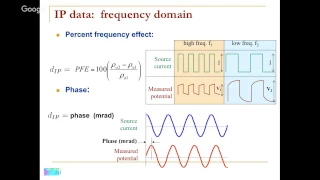
So
it's
maybe
showing
move
it
better
here.
So
here's
our
current
I
of
G,
here's
the
received
voltage
looks
like
this.
It's
got
whatever
Act
it
has,
and
we
notice
that
it's
got
a
phase
shift
here
between
this
and
this.
So
that's
also
indicating
wait
a
minute,
there's
some
kind
of
a
delay.
That's
going
on
in
that
that
delay
is
representative
of
how
much
time
it's
taking
for
those
charges
to.
A
So
that
would
be
a
datum,
and
the
final
datum
that
we
have
is
something
called
a
percent
frequency
effect
and
what
that
does
is
it.
It
works
with
a
current
that
has
got
kind
of
a
fast.
Switching,
so
by
taking
a
current
source
and
I
do
make
it
positive
and
the
negative
positive
negative
that
I
do
it
at
a
very
small
time.
Scale
then
what's
gonna
happen
here
is
the
moment.
I
turn
this
on
those
that
over
voltage
is
going
to
start
to
build
up.
A
So
it's
good
come
up
this
way,
but
it
never
gets
a
chance
to
come
up
to
its
final
value
because
now
I'm
switching
it
off
in
the
other
direction,
so
it
gets
switched
off
and
it
comes
down
like
this
and
then
kind
of
reaches
like
that.
So
the
point
is
I
get
to
have
a
certain
upper
value
here,
that's
obtained
before
I
switch
things
up.
A
So
if
I
change
things
around
and
I
say,
oh
I'm
gonna
have
a
current
that
his
you
know
it's
on
for
much
longer
length
of
time,
then
that
over
voltage
has
more
time
to
build
up.
So
the
Chris
charges
build
up
and
I
actually
received
this
point
here
and
then
I
go
back
down.
So
you
see
that
this
number
up
here
is
actually
larger
there.
This
one.
A
So
if
we
take
these
these
numbers
here,
we've
got
an
apparent
reason.
Stivity
from
here
we've
got
an
apparent
resistivity
from
here.
I
can
subtract
them
and
normalize
by
1,
multiplied
by
100
and
I
get
what's
called
a
percent
frequency
effect,
and
so
that's
another
IP
data.
So
you
can
see
there's
a
whole
bunch
of
ways
of
actually
getting
something
out.
That's
representative
of
the
idea
that
wait
a
minute
those
charges
being
being
built
up
here
so
I've
got
ground.
A
A
A
So
this
is
exactly
what
we
had
before
so
remember
how
we
did
that
if,
if
you've
got,
this
was
a
dipole
dipole.
That's
when
we've
got
a
dipole
current
source
at
a
dipole
potential
field,
and
then
we
wanted
to
plot
that
on
plane.
So
we
just
did
these
45-degree
angles
and
then
we
looked
at
where
they're
intersecting
and
they
said
ok
I'm,
going
to
plot
the
datum
there
for
the
DC
resistivity.
We
plotted
the
apparent
rescinded.
A
So
we
that
voltage,
/
dance
and
for
chargeability
we're
just
going
to
take
whatever
number
we
get
there
and
plot
the
chargeability.
Yet
so
it's
going
to
look
perhaps
somewhat
similar,
but
units
are
going
to
be
quite
different
and
the
interpretation
is
what
this
one
and
then
again
for
the
for
building
up
the
pseudo
section.
Never
did
that
and
it's
it's
kind
of
sounding
and
profiling
mode,
where
we
just
kind
of
continue
moving
the
whole
system
along
separating
transmitters
and
receivers,
taking
the
apparently
sensitivities
and
bottom-up.
A
A
A
So
if
I
go
ahead
and
I
do
that
same
dipole-dipole
survey
over
top
of
here
want
my
suit
of
section
now
I'm
going
to
get
out,
you
know
a
picture
that
looks
like
that
and
as
we
end
the
deep-sea,
you
see
that
okay,
it's
it's
got
some
information,
perhaps
both
this
with
exactly
the
same.
But
you
know
there's
a
peak
of
chargeability
happening
right
here:
yeah
baby,
if
I
drill
down
here
I
might
hit
something.
This
axis
here
is
not
true
depth,
it's
a
kind
of
like
a
pseudo
death.
A
A
A
Again,
if
we
add
little
bits
of
stuff
now,
these
things
are
all
the
same:
conductivity
no
change,
but
they
are.
You
have
different
charms
abilities
and
get
clays
graphite
sulfides.
Those
are
the
big
ones.
That's
from
your
perspective
plays
our
city
and
something
it
looked
like
that.
Then
now
you're
see
this
section
just
gets
all,
but
you
can't
you
just
can't
see.
A
And
one
final
one
and
it's
got
another
complication,
because
if
you
have
kapag
rafi
on
any
of
these
surveys
that
it
turns
out,
the
topography
makes
a
big
difference
in
the
safe.
You
know,
and
if
you've
had
a
sharp
of
body
here
and
one
in
charge
of
the
body
he
with
a
slight
surface
charge
ability
your
suitor
section
looks,
looks
like
this.
This
suitor
section
is,
it
knows
a
picture.
The
data
is
absolutely
nothing
to
do
geologically
with.
What's
going
on
here
like
yours,
there's
no.
A
So
now
we're
back
to
the
same
situation
that
we
were
before
in
the
DC
resistivity,
and
that
is
that
you,
basically
we
don't
have
any
choice
except
to
kind
of
invert.
The
data
I
didn't
really
get
a
chance
to
go
through
this.
The
last
time
and
I
don't
have
another
chance.
This
time.
I
just
put
this
up
just
to
kind
of
give
you
a
feeling
that
when
you
invert
data,
there's
actually
quite
a
few
steps
that
you
need
to
to
go
through,
but
the
basic
essence
is
in
Beckford
for
the
to
deep.
A
A
A
J
ADA
is
equal
to
D,
so
Deena's
like
data
and
is
our
chargeability
model
and
J
is
a
matrix.
So
if
I
was
a
bit
more
explicit
and
I
said,
oh,
that's
that's
about
capital
m
and
elements.
So
then
a
defector
is
got
no
size.
Pam
dee
has
got
a
size
in
so
J.
The
matrix
J
has
got
to
be
an
N
by
M
matrix
right,
so
that
he's
got
J
is
n
by
M.
A
So,
in
our
case,
these
data
could
be
anything
that
we
had
before,
so
they
could
be
millivolts
per
vault.
It
could
be
milliseconds,
they
could
be
PA
fees,
they
could
be
milliradians
that
doesn't
matter
we
take
whatever
those
data
are
and
we
compute.
What
we
need
to
do
is
to
compute
this
sensitivity,
function.
A
Here's
our
current
and
here's
our
potentials
and
we're
going
to
collect
these
data
as
well
as
some
supply
P
data
and
we're
going
to
try
to
invert
those
things.
So
the
very
first
thing
is
what
we
did
yesterday
is
we
took
these
potentials
converting
them
to
pair
resistivities,
and
then
we
tried
to
find
a
resistivity
or
conductivity
structure
that
gave
rise
to
those
data.
So
that's
the
DC
experiences.
We
now
have
a
a
map
of
electrical
conductivity
or
electrical
resistor
good.
A
The
next
step
for
working
with
the
IP
is
that
we
actually
need
to
use
this
guy
this
conductivity
structure
and
we're
going
to
use
that
to
compute
this
sensitivity.
Quantity
here
J,
so
that
my
mapping
be
like
between
the
data
and
the
charge
abilities
is
the
sensitivity,
function
and
I
actually
need
to
have
the
conductivity
to
do
that,
and
then
once
I've
got
that
then
I'm
back
to
solving
that
problem,
and
now
I
can
solve
for
the
charge
ability.
A
So
it's
always
a
two-step
process,
and
if
you,
if
you're
connected
with
anybody,
who's
doing
dcpip
experiments,
they're
always
going
to
do
it
in
two
steps.
They're
going
to
take.
Take
the
voltages,
compute,
the
conductivity
and
they're,
going
to
take
that
conductivity
sensitivity,
and
it's
all
that
chargeability.
A
So
always
the
always
the
same
thing
so
just
to
show
you
how
that
how
that
can
work
in
this
particular
case.
So,
let's
take
that
charge
ability
model,
here's
our
our
pseudo
section.
If
we
take
this
and
invert
the
charge
ability,
that's
what
we
get.
So
this
is
great
right.
We've
got
a
nice
localized
body
wearing
the
where
the
prison
is
it's
not
nearly
as
sharp,
but
within
the
context
of
our
inversion,
we're
actually
asking
for
something
that
was
a
bit
smooth.
A
So
this
is
this
is
pretty
nice,
it's
it's
at
about
the
right
location,
both
in
depth
and
certainly
horizontally,
and
if
we
take
this
and
we
forward
model
it,
that's
our
data,
that's
our
predicted
data,
and
so
this
predicted
data
is
a
pretty
good
match
to
the
observed
data.
So
mission
accomplished
right,
taking
our
data
inverted
about
something
finds
that
it
reproduces
the
satisfaction.
A
Go
down
to
this
guy,
it's
got
more
stuff
there.
Now
the
pseudo
section
is
completely
uninterpretable.
You
can't
can't
see
anything
there,
but
if
you
go
ahead
and
invert
them,
you
can
start
to
see.
First
of
all,
I've
got
my
prism,
but
even
more
than
that,
I've
got
these
little
guys
that
are
sitting
up
here.
Oh
my
pieces
of
graphite,
my
predicted
date
look
like
that
which
is
like
that.
A
A
What's
going
on
this
guy
stuff,
you
look
at
it
and
very
often
you
can't
tell
anything
so
it's
only
after
you
unravel
it
with
inversion,
sometimes,
but
between
the
observed
and
predicted
data,
and
this
one
is
specific,
especially
interesting,
because
they've
got
this
charcoal
body
here
and
another
charge
of
a
body
gear,
and
if
you
generate
the
pseudo
section
of
that,
it
actually
looks
like.
Oh
I've
got
a
great
big
chargeable
body
here.
A
Well,
if
you
wind
the
clock
back
a
couple
of
decades
ago,
people
would
have
looked
at
this
and
said.
Terrific.
Look
at
that!
There's
a
great
big!
You
know
charge
of
a
body,
it's
probably
a
sulfide
down
there.
That's
spotted
going
right
down
like
that
and
that
would
have
drilled
right
down
through
here.
So
they
missed
easily
to
miss
everything
just
by
kind
of
making
some
quick
opinion
on
that.
A
But
if
you
take
that
go
ahead
and
you
the
birthday,
this
is
what
you
see
see
you
got
now
you
have
charge
of
a
park
here
and
truck
for
life.
You
don't
see
all
this
stuff,
that's
really
going
down
here
and
that's
simply
because
the
experiment
was
such
that
we
weren't
really
driving
currents
down
here.
So
we
didn't
really
ignite
this
part
of
the
of
the
object
completely.
So
there's
not
very
much
information
coming
from
here,
so
you
do.
A
The
inversion
doesn't
have
to
put
anything
there
and
you
end
up
with
something
like
this,
and
so
when
we
hear
you
know
you're
kind
of
smeared,
oh,
but
from
the
point
of
view
of
geologic
interpretation,
you
now
have
something
you've
got
a
potty
here
got
a
buddy
here
know.
If
you
drill
in
here
drilled
in
here,
you'd
be
very
happy.
A
So
I
want
to
go
back
to
this
example
that
I
had
talked
about
last
last
day
because
we
did
the
DC
resistivity
and
we
ended
up
with
a
great
geologic
model,
but
one
that
really
wasn't
of
particularly
interest,
interesting
from
mineralization,
so
just
to
refresh
your
eminence
what
we
had
so
this
was
in
northern
Australia.
So
this
is
like
three
half
kilometers
by
a
couple
of
kilometers
there's
ten
lines
of
data
and
the
data
were
either
pole,
dipole
or
dipole
pole.
A
A
So
just
igniting
the
earth
from
different
angles
gives
rise
to
different
datasets.
But
the
thing
with
all
of
these
pseudo
sections
is
that
there's
only
one
earth
model
there
all
right,
so
all
of
these
things
are
somehow
kind
of
encoded
information
about
parts
of
that
model.
What
we
really
want
to
do
is
sort
of
combine
them
all
together,
and
so
we
did
that
through
the
conversion.
A
A
We
progressively
made
every
pixel
that
was
less
than
a
certain
value
made
that
completely
transparent.
So
in
the
end,
the
only
thing
that
we
end
up
with
is
this
this
conductor
here,
and
that
was
that
black
shale
unit,
which
geologically
is
interesting
for
the
point
of
view
of
mineral
exploration.
It
was
no
interest
if
we
kind
of
took
a
like
a
snapshot
through
at
some
level.
Some
planning
in
that
you
can
see
how
this
big,
really
conductive
coaster.
A
A
Kind
of
comes
like
this,
so
the
numbers
that
we're
seeing
you
here
for
charge
ability,
like
they're,
really
small
compared
to
these
guys
here
so
because
the
numbers
are
small.
When
you
get
to
really
large
offsets
between
the
transmitter
receiver,
the
signals
are
so
small,
it's
basically
noise,
so
these
have
to
get
cut
off
other
than
that
it's
the
same
suitor
section.
So
again,
this
was
a
dipole
pole.
A
A
A
A
So
what
we
see
is
that
we've
got
a
nice
even
nation
of
this.
If
we
take
a
look
at
the
electrical
conductivity,
but
by
night
there
was
some
manifestation
in
here
about
kind
of
an
if
you
mid-range
intermediate
sort
of
conductivity,
which
is
what
they
felt.
The
mineralization
should
be
so
mineralization
to
be
kind
of
moderate
conductivity,
not
nearly
as
much
as
this
background
and
quite
chargeable,
compared
to
the
background
and.
A
A
A
I
I,
don't
know
how
you
tell
ya
that
they
have
to.
They
should
provide
that
information.
What
the
data
acquisition
is
to
get
those
okay,
so
that
is
basically
the
end
of
the
material
for
the
course
they
as
we
go
through
so
Friday
we'll
have
a
a
team-based
learning,
so
it's
gonna
be
based
on
this
material,
so
the
PC
resistivity,
the
IP
for
waste
dumps
that's
becoming
more
and
more
common.
These
days,
there's
all
kinds
of
places
that
people
are.
You
know
ducked
garbage
there
now
degrading
and
stuff.
A
That's
getting
out
leaching
into
local
groundwater
supplies.
It's
become
up.
You
know
a
big
problem
and
I'm
starting
to
get
an
IP
is
probably
one
of
the
most
effective
ways
of
better
understanding
something
about
that
weight.
Stuff.
So
I
think
you'll
be
really
interested
in
this
and
well
kind
of
ties.
What
we've
just
talked
about:
yeah
Monday,
we'll
do
a
quiz
and
then
that
kind
of
finishes
up
all
of
that
technical,
Carol
and
I
got
Wednesday
and
Friday
to
kind
of
do
some
recapping.