►
From YouTube: Houston Course Day 4: Afternoon
Description
No description was provided for this meeting.
If this is YOUR meeting, an easy way to fix this is to add a description to your video, wherever mtngs.io found it (probably YouTube).
A
A
You're
going
to
demonstrate
yeah
so
just
to
remind
you
where
we
are
so
all
the
things
that
we're
going
to
be
looking
at
we're
going
to.
We
use
the
word
when
we
use
the
word
model,
we're
going
to
be
talking
about.
You
know
whatever
function,
we're
trying
to
find
or
set
of
parameters,
the
context
and
inversion,
that's
what
the
might
use
or
the
context
for
that
particular
word.
A
The
physics
that
you
are
working
with
is
going
to
be
described
for
a
linear
problem
by
these
kernel
functions
and
each
datum
that
you
have
can
be
thought
of.
As
you
know,
an
inner
product
of
your
model
with
a
kernel
function,
so
that
gives
you
your
your
gayness
I,
showed
you
a
little
bit
through
the
app,
so
you've
got
capabilities
of
generating
some
combination
of
a
Gaussian
and
boxcar,
and
then,
when
you
have
this
specify,
you
also
specify
your
kernels.
That
gives
you
your
data
and
then
you
can
add
some
noise
to
it.
C
A
A
D
C
A
A
You
have
the
standard
deviation
of
your
go
see,
so
this
is
Gaussian
noise,
that's
got
zero
mean
and
standard
deviation
epsilon.
So
you
know
it
kind
of
looks
like
this.
So
zero
me
standard
deviation
epsilon.
So
this
is
sort
of
plus
or
minus
one.
Epsilon
sub
gives
you
the
width
of
the
Gaussian,
and
so
then
KS
make
noise.
We
we
draw
a
sample
from
this
and
added
to
that,
the
standard
deviation.
Epsilon
is
some
sort
of
percentage.
C
A
A
A
Okay,
so
let's,
let's
actually
take
this
a
little
bit
more
slowly.
We're
gonna
set
up
set
up
the
inverse
probability.
So
now
we've
got
our
observations.
They're
contaminated
with
noise,
we're
going
to
estimate
an
uncertainty
for
those.
We
have
the
ability
to
do
the
forward
modelling,
and
now
we
want
to
do
the
inverse
problem,
we're
going
back
from
the
data
to
the
model
space
and
for
this
linear
problem.
We
just
write
the
data
as
GM
is
equal
to
D
and
important
thing
here.
A
So
when
we're
working
with
an
inverse
problem,
we
saw
before
we're
actually
trying
to
find
a
function
and
a
function
has
infinitely
many
degrees
of
freedom,
we're
going
to
have
a
representation
of
that
with
respect
to
a
certain
number
itself,
but
that
number
of
cells
is
much
much
larger
than
the
number
of
data
that
you're.
So
it's
quite
an
underdetermined
system.
A
Some
noise
epsilon
and
we're
going
to
represent
that
noise
with
as
gaussian
standard,
deviation,
epsilon
J,
and
so
there
are
there
for
our
misfit
measures.
Is
this
one?
It's
going
to
be
the
difference
between
the
observed
and
the
predictive
value
divided
by
our
estimated
uncertainty,
so
the
quantity
that
we're
going
to
estimate
is
the
standard
deviation
of
the
of
the
observation
and
we're.
A
If
the
data
errors
are
Gaussian,
zero
mean
and
so
particularly
well
the
unit
standard
nation.
So
if
there's
zero
mean
with
unit
staff
deviation
and
the
division
by
epsilon
here
tries
to
accommodate
that,
then
we've
got
a
statistical
quantity
here
for
which
there's
an
expected
value.
So
the
expected
value
of
this
quantity
here
is
approximately
equal
to
the
number
of
data.
So
that's
important
because
we
not
only
need
to
have
a
measure
of
this,
but
we
need
to
have
a
criterion
for
deciding
okay.
When
are
we
kind
of?
A
A
A
A
A
So,
as
I
said,
here's
our
here's,
our
misfit
criteria,
we've
already
said
there
should
be
an
expected
value
of
this.
Maybe
is
something
in
the
order
of
an,
but
if
we
forget
about
that
first
for
the
moment
and
just
try
to
see
okay,
let's
just
make
this
as
small
as
possible,
and
that
brings
us
to
the
point
where
we
were
just
prior
to
maybe
for
lunch
and
that's
what
happened
with
the
conversion
app,
and
you
saw
that
as
we
fit
the
data
better
and
better.
A
B
A
Is
that
there's
non
uniqueness
in
this
problem
and
there's
there's
a
couple
reasons
for
non
uniqueness:
I
mean
sometimes
there
might
be
just
playing
physical
basis
for
that,
for
anybody,
who's
done
potential
fields,
and
since
you
know
that
if
you
take
gravity
values
over
surface
or
magnetic
values
over
your
surface,
that
you
could
reproduce
those
observations.
Just
by
having
an
infant
test
within.
C
A
A
A
And
D
Series
is
dedicated
there's.
This
is
an
example.
We
actually
put
this
together
two
years
ago
to
quantify
depth
of
investigation.
The
model
here
is
as
follows:
the
red
is
our
conductive
units,
so
there's
three
red
units
up
here,
there's
a
long
vertical
conductor
here,
there's
a
short
conductor
here
and
there's
a
resistive
body
here,
there's
a
ladder
of
conductivity
contrast.
So
this
is
more
of
a
conductive
on
here,
more
resistive
and
then
Barry
a
year,
there's
a
changing
over
burden
as
well
as
as
a
conductor.
So
it's
a
fairly
complicated
system.
A
A
A
B
A
B
A
A
A
E
A
A
B
A
A
A
A
Okay,
so
that's
what
we're
faced
with
that's
a
fundamental
non
uniqueness!
That's
going
to
happen
in
every
universe,
problem
that
that
you
work
with,
and
so
you
need
to
think
about
this
right
up
front.
So
the
idea
of
you
trying
to
decide
what
you
know
kind
of
while
or
how
do
I?
How
do
I
select
from
an
infinitely
many
of
really
crazy
variable
models,
otherwise,
like
what
that
is
that.
E
A
C
A
A
E
A
A
So
now
we
come
to
the
ok
there's
many
solutions.
I
was
kicked
one
out
of
that
and
we
we
basically
need
to
have
extra
knowledge
and
extra
information,
and
that
could
come
from
a
whole
bunch
of
ways
is
there
could
be
geophysical?
Knowledge
may
be,
you
know,
the
values
are
positive
or
within
some
boxes,
so
you've
got
the
physical
model.
There
you
go
say
seismic
velocity
try
to
be
think
I'm,
a
positive,
negative,
velocities
and
they're
certain
crackers.
Okay.
So
that's
that's
a
possible
thing.
A
A
The
other
is
is
more
of
a
structural,
more
of
a
kind
of
a
philosophical
idea
about
kind
of
what
you
want
to
yeah
I
mean
you.
You
obviously
have
the
choice
of
making
something
that's
complicated
or
you
can
make
it
something.
That's
simple!
So
the
idea
is
like
okay.
Well,
if
you,
if
you
have
a
solution
with
thirty.
A
A
C
A
I
can
I
find
something
that
you
know.
It's
got
a
scaling
longer
longer
than
this
or
maybe
there's
structural
constraints.
You
simply
know
that.
Okay,
there
should
be
a
fault
in
this
area,
so
these
are
like
the
kinds
of
things
that
you
need
to
now
start
to
think
about
and
to
accumulate
before
you
even
really
start
to
press
the
button
on
run
the
inverse
problem,
let's,
let's
just
bring
together
all
the
a
priori
knowledge
that
I
already
have
and
then
step
use
that
to
help
set
up
a
problem.
C
A
About
this
problem
of
trying
to
pick
a
single
solution
from
infinitely
many
possibilities,
and
sometimes
this
kind
of
resonates
and
supposes
that
you
know
you
use
everybody
here
and
I'm
I'm
faced
with
a
you,
live
with
a
solution
I'm
trying
to
find
okay.
So
here's
my
question
find
find
a
person
in
the
room
right
so
that
there's
many
answers
to
this
right.
So
each
one
of
you
could
be
potentially
a
solution
and
that's
not
enough
information
to
go
on
so
I
need.
C
A
A
A
A
G
Many
ways
this
inversion
problem:
it
has
two
kinds
right.
One
of
us
the
one
year
showed
shown
us.
That's.
The
number
of
unknowns
is
greater
of
dependent.
Number
of
equations
means
X
plus
y
equals
one
equation
for
two
notes,
but
I
could
maybe
go
smooth
sighs
the
poor
usually
have
the
other
opposites
when
you
lower
size
experience.
G
If
you
take
all
the
number
of
data
that
you
have
the
number
of
braces,
the
number
of
samples
for
trace
all
the
information
that
have
the
number
of
unknowns
is
much
less
in
the
number
of
information
that
we
have
so
the
problem
user.
It's
not
that
we
have
infinite
solutions
that
we
don't
have
any
solutions
at
all,
because
the
number
of
we
don't
have
one
single
solution
that
fits
scimitars
of
the
label.
G
So
we
need
to
move
to
like
at
least
we're
approaching
something
that
okay,
we
can't
have
one
model
that
fits
all
equations
because
have
too
many
too
many
operations
for
few
unknowns,
and
then
we
need
to
choose
one
model.
We
select
one
object,
exhausted,
that's,
okay,
it
doesn't
fix
all
equations,
but
the
distance
from
this
evolution
among
our
equations,
the
minimum
possible.
That's
exactly
the
opposite
that
this
kind
of
immersion
problem.
That's
phenomenal!
G
A
First
of
all,
when
you,
when
you're
setting
this
problem,
you're
you're
going
to
still
be
dividing
things
into
into
cells
right
so
already
that's
a
that's
a
parameterization.
If
you
were
really
trying
to
find
a
function
and
those
cells
should
be
really
small
and
you
you
know
to
help
solve
that
inverse
problem,
then
you
probably
would
have
more
unknown
data.
The
other
is
that
even
when
you
have
parameterised
like
this,
you
say
well,
I
got
got
lots
of
data
I'm
sure
you
might
have
like
the
total
number.
A
A
C
A
A
C
A
So
let's
set
this
example
here,
just
a
bit
more
complicated,
so
it's
a
four
parameter
problem
got
m1
through
m4
and
about
Takeda.
So
this
combination
gives
six.
This
combination
gives
two,
so
they
got
four
unknowns
to
two
data.
So
there
is
not
any
solutions
right
then.
So
here's
here's
four
solutions.
So
there's
one
that's
just
constant
and
then
there's
so.
A
One
possibility
is
that
I
could
just
basically
make
a
ruler
that
kind
of
measures
the
many
measures
the
size.
So
we
need
to
have
a
ruler
that
could
measure
your
length
or
some
characteristic
of
that
we're
going
to
refer
to
that
that's
the
spice.
So
this
is
going
to
be
or
metric
thing.
Everybody
tried
to
minimize
and
then
it's
a
question
of
what
this
is.
So,
for
instance,
it
could
be
this
moment
like
what
what's
the
sum
of
squares
all
of
the
elements.
A
So
if
we
just
looked
at
something
something
like
this,
then
that
would
be
one
way
that
we
could
judge
things,
and
so
that's
just
looking
essentially
a
kind
of
like
the
energy.
The
other
possibility
is
that
we
could
look
at
the
variation
of
the
elements
or
the
try
to
minimize
the
distance
between
successive
elements.
Let
techniques
a
solution
that
sort
of
smooth
or
black.
If
you
can
minimize
first
term
the
first
order
derivative,
so
this
would
be
the
sum
of
squares
of
differences
between
between
two
adjacent
elements.
A
A
This
answered
B
as
a
value
except
four
to
nine,
and
that
is
shown
by
this
this
curve.
So,
where
we're
looking
at
these
successive
orange
points
here
as
being
solution,
if
we
chose
a
different
metric
but
say
we
chose
this
smoothness
month,
we're
minimizing
the
variation
these
successive
elements.
In
that
case
the.
A
A
A
So
one
of
the
things
that
you
can
work
with
well,
there's
a
whole
host
of
them
in
the
app
that
you
can
work
with.
These
are
ones
that
are
available.
So
you
could
minimize
the
square
of
the
function
you
could
minimize
it
could
introduce
a
reference
model
and
then
minimize
the
deviation
of
the
bottle
from
that
from
that
reference.
But
that
could
be
something
you
could
actually
ask
for
just
something
or
smooth
where
you're
minimizing
the
energy
of
the
derivative,
and
you
can.
A
C
A
Morning
was
showing
in
the
in
version
of
the
empty
data
and
CSF
data.
You
know
successive
inversions,
where
you
know
you
invert,
one
dataset,
you
get,
you
get
a
model,
and
then
you
use
that
as
initial
and
reference
model
for
another
one,
and
then
you
can
kind
of
iterate
iterate
your
way
through
so
kind
of
successive
iterations
and
here's
where
that
reference
model.
G
So
I
always
go
home,
brace
precisely
because
I
will
always
size,
but
in
silently
trying
to
get
some
version.
Usually
we
am
yes
and
other
models
we
used
to
wear
in
l1
North
then
introduced
a
sparse
sparse.
So
we
cannot
kind
of
gain
resolution
with
the
Dallas
boots,
all
right,
very
everyone,
no,
no
as
well
yeah.
A
A
C
A
L0
normal
give
you
the
fewest
number
of
elements.
No
one
will
also
give
you
something
as
farce.
L
too
will
tended
with
just
mean
things
I
admitted,
so
you
really
don't
need
a
lot
of.
In
fact,
you
want
to
have
as
few
terms
here
as
things
quickly
get
getting
complicated,
but
not
necessarily
complicated.
It's
just
that
you've
got.
We've
got
too
many
buttons
to
adjust.
A
A
That,
but
now,
okay,
who
do
you
want
to
wait
more?
Do
you
want
it
to
be
closer
to
wait
that
makes
it
closest
to
a
reference
model?
Is
that
the
more
important
or
you
want
smoothness
to
be
more
important,
and
those
are
parameters
that
are
generally
subjected,
there's
not
any
way
of
mathematically
determining
what
they
they
should
be?
A
Okay,
so
now
we
we
said,
there's
two
things
that
that
we've
got.
We
want
to
find
the
solution
that
produces
a
misfit
to
the
data,
that's
approximately
equal
to
some
target
misfit
and,
as
we
saw
this
morning,
we
don't
necessarily
want
to
make
that
as
small
as
possible,
because
if
we
do
we're
going
to
be
adding
a
lot
of
structure,
that's
just
unicorn
stuff,
and
we
also
want
to
minimize
this
model
objective
function
that
we've
got
so
that
we
find
the
smallest
element.
E
A
All
the
candidates
here,
so
there
is
way
somehow
to
do
that.
Well,
we're
going
to
recast
the
inverse
problem
as
optimization
problem
where
we
actually
minimize
the
sum
of
these
two.
So
we're
going
to
minimize
a
5
which
is
equal
to
misfit
plus
beta
times.
Our
objective
function
and
beta
is
just
is
a
trade
on
parameters.
C
A
Here's
here's,
if
our
attempt
to
put
everything
in
a
totally
different
context,
but
still
show
the
same
basic
elements.
So
imagine
that
you're
traveling
from
point
A
to
point
B.
This
light
was
made
when
we
were
in
Vancouver,
so
we're
great
to
travel
from
Vancouver
up
to
Calgary,
and
we've
got
an
optimization
problem
here
in
the
sense
that
we
want.
A
To
minimize
the
fuel
consumption,
so
we
don't
want
to
be
burdening
if
you
ever
get
a
an
electric
car
from
Tesla
or
something
did
you.
These
things
are
actually
going
to
be
really
important
because
you
only
have
a
certain
distance,
pre
charging
stations
and
you're
whining.
You
don't
want
to
put
your
car
in
the
fastest
speed
possible
because
you
might
not.
E
A
So
if
a
is
equal
to
zero,
okay,
then
we're
just
minimizing
the
time,
so
we're
just
don't
care
at
all
about
the
fuel
we
just
go
as
fast
as
we
possibly
can
and
do
that
on
this
axis
here,
your
time
on
the
road
and
on
this
axis,
we've
got
the
old
assumption.
So
when
theta
is
equal
to
zero,
we're
kind
of
out
here,
we've
got
big
fuel
consumption
and
our
time
on
the
road
is
the
other
end
of
the
scale
is
when
beta
is
really
more
okay,
and
we
want
to
minimize
the.
A
C
C
A
That
would
be
kind
of
our
guitar
good,
and
that
would
put
us
at
this
point
here.
So
as
we
change
data
from
something
that's
really
big
to
something.
That's
really
small,
then
we're
constantly
kind
of
favoring,
this
particular
route
here
and
at
this
particular
point
we
actually
hit
a
target
value
and
we
stayed
so
that
we're
going
to
do
the
same
thing
now
with
the
interest
problem
and
the
beta
is
plays
exactly
that
same
role.
So
from
our
inverse
problem.
We're
going
to
minimize
the
sum
of
misfit
plus
beta
yeah,
so.
B
A
Rate
of
as
every
time
we
change
beta
beta
starts
at
infinity,
then
we're
going
to
be
hot
here
as
beta
gets
smaller.
We
progressively
flow
down
this
curve,
and
we
have
down
here
sounds
funny:
okay,
which
buffet
do
we
use
well,
we
do
have
one
thing
that
we've
worked
with,
and
that
is
we
generated
this
misfit
function
and
within
that
we
estimated
the
standard
deviations
of
theirs
so
that
the
expected
value
of.
A
G
The
immersion
proms
that
I'm
used
to
do
I
agree
with
all
the
points
that
you
image.
Okay,
the
number
of
renounce
does
depend,
of
course,
on
the
sound,
so
it
may
find
the
number
of
unknown
the
number
of
parts
of
that
we
have
so
never.
But
you
know
Mathematica
just
put
in
the
same
way
that
you,
okay,
X,
plus
y,
equals
two.
Then
we
have
this
linear
function
and
any
white
can
have
a
solution.
Yeah
their
problems
are
I
used
to
deal
in
my
they'll
jump.
It's
exactly
that.
I
have
one.
G
G
Okay,
so
this
one's
the
best
one
but
then
I
have
a
third
equation
view,
so
it
I
don't
have
this
common
point.
Okay,
so
I
have
this
three
equation.
So
maybe
I
to
the
point
like
here
yeah
and
it's
it's
a
solution.
They
waited
okay
I
want
to
find
out
a
solution
for
anyone.
But
of
course
me
one
of
these
so
norms,
one
of
this
crusade-
okay,
maybe
they
the
minimum
distance
between
the
solution.
Amin
Amin,
we
interviewed
to
meet
expire,
our
criteria
to
choose
one.
C
G
Lists
are
approaching
in
gel
faces,
taking
particular
luminosity
Asian
like
300.
The
range
between
the
number
one
number
in
other
notes
and
think
about
the
size
of
experience
of
okay,
also
know
the
ocean
bottom,
so
I
haven't
used.
One
thousand
notes:
I
have
a
huge
number
of
shots
for
each
shots.
I
have
for
silent
race
for
companies
for
each
note,
its
trace,
like
oh
thanks,
icons
with
a
zoom
in
second
sample,
so
the
number
of
beta
is
actually
number
of
samples.
So
you
multiply
the
number
of
shots.
G
The
number
of
receivers,
the
number
of
samples
in
each
trace
that
give
us
a
big
ignorant
as
the
data
that
we
have
the
number
of
unknowns,
the
size,
mall
and
usually
the
sizing
we
reverse
for,
like
a
25
by
25
by
5
meters.
That's
the
volume
one
possible!
You
know.
If
you
take
this
busiest
one
unknown
customer
for
one
parameters,
the
whole
model,
it
will
give
us
like
a
300,
more
data
than
the
number
of
and
in.
G
Well,
even
if
that's
like
quite
a
number
from
notes
or
three,
so
even
though
we
have
like
100
more
data,
then
unknown,
that's
the
usual
okay,
of
course,
as
you
said,
if
I
set
my
cell
so
1
meter
by
1
meter
by
1,
meter
danik
and
moves
to
the
opposite
side
of
theta,
0
and
I'm
for
know,
we
may
be
great,
but
that's
not
the
way.
We
usually
don't
think
so.
Nice.
A
But
suppose
I
take
that
same
that
same
thing
and
I
think
now
I'm
going
to
parameterize
it
different
instead
of
having
other
layers
I'm
gonna
50,
and
now
we
can
push
it
as
far
as
and
then
let's
reduce
it
even
more.
Instead
of
having
50
Larry,
let's
have
five
layers.
Okay,
now
now
we're
not
going
to
get
crazy,
crazy
solutions,
we're
going
to
be
hitting
and
resolved.
That
has
something.
C
A
F
A
E
A
C
A
That
is
when
you
do
your
problem,
even
though
you
cannot
fit
the
data
and
you
try
to
fit
the
data
as
well
as
you
possibly
can.
The
question
is
whether
the
structure
that
you
get
out
is
actually
adequate
for.
What
you
need,
or
is
you
know,
should
you
be
putting
in
your
like
something
that
is
makes
it
more
smooth.
C
G
A
To
okay,
so
if
Airport,
you
still
have
it,
sometimes
you
can
refer
to
as
under
constraint.
Problem
right,
so
you
you
technically
have
more.
Then
you
have
unknowns,
but
still
there's
a
lot
of
latitude
in
there
to
get
many
different
kinds
of
functions
of,
and
some
of
them
could
be
quite
wrong.
Some
of
them
could
be
right
and
you
need
to
have
some
extra
regularization
so
and
the
other
way
of
kind
thing
about
that
is
that
oh
yeah
I
do
have.
A
A
If
X,
so
this
is
so
what's
the
images
like
these
there's
quite
a
ways
that
you
can
address
this
problem,
one
that
we've
implemented
a
lot
in
our
work
is
actually
iteratively
solve
the
problem,
but
at
each
iteration
will
reduce
the
value
of
betas,
will
kind
of
do
a
beta
cooling.
So
in
that
case,
you'll
start
at
a
high
value
of
beta,
a
very
little
structure
and
just
gradually
reduce
beta
the
data
better
and
better.
At
some
point,
you
just
read
your
fitting
well
enough
or.
C
A
I
think
if
you
consider
that
a
complete
size,
maybe
on
a
seismic
migration,
is
it's
effectively
one.
The
iteration
in
a
full
conversion
quite
quickly
appreciate
that
it
is
going
to
be
hard
to
do
a
large
number
I'm,
not
sure
where
the
seismic
industry
is
with
respect
to
that
you're,
you're
kind
of
a
that's
extreme
and
though.
F
So
here
we
got
the
people
set
up
in
Sweeney
and
the
model
is
hundred,
for
instance.
Now,
let's
say
we
got
to
speak
P
model
and
then
beta
is
60
and
it'll.
Give
you
an
error,
that's
fine!
You
don't
really
have
to
stop
there
and
then
just
run.
The
other.
App
then
can
share
the
data
that
looks
like
so
you
got.
C
E
F
Here,
if
you
say,
if
I,
if
the
Run
button
is
clicked,
that
means
every
click,
it
runs
the
a
person
again
so
I'm
going
to
activate
that
now.
I'm
you're
in
this
I'm
sort
of
like
a
coring
mo
so
yeah.
So
we
got.
We
actually
got
thirty
to
forty
iteration.
You
want
to
explore
how
they
did
inversion,
so
I
think
that's
yeah
I'll
just
walk
through,
though
yeah.
A
C
A
G
C
A
C
F
A
A
A
A
A
A
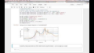
Here's
now
we're
gonna
play
around
with
this
particular
this
structure,
we're
up
here
on
this
pig
knocker.
So
what's
going
to
happen,
is
we're
going
to
progressively
reduce
the
value
of
beta
and
each
point
we
solve
not
linear,
linear
problem
get
a
model
of
the
data,
so
we
have
the
observed
of
the
date
of
misfit
and
then
there's
also
a
model
norm,
the
rank
of
your
people
that
have
to
thought
before.
So
what
we're
plotting
on
here
is
by
M.
So
this
is
this.
A
A
A
There
sorry
I
can't
hear
when
we
actually
plot
the
the
taken
off
curve,
where
we
bought
five
years
a
function
of
him.
Then
that
turns
out
to
be
a
place
that
you
could
choose
as
sometimes
an
optimum
value
at
this
point
here.
We're
just
kind
of
continuing
to
reduce
the
misfit
and
the
bottom
arm
is
gradually
increasing
and
we'll
see
how
bad
it
gets.
E
C
A
A
E
A
So
that's
at
this
sort
of
target
value
here,
and
that
would
be
maybe
a
first
estimate
of
you
know
getting
our
solution.
That
is
your
fitting.
The
data
to
about
kind
of
what
you
wanted
you're,
also
getting
might
be
able
to
do
a
little
bit
better,
estimating
missed
it
just
on
that
approximation
of
the
expectedness
fitness.
It's
a
good
story
thanks,
but
we
really
want
to
see
if
we
can
push
the
data,
maybe
a
little
bit
more.
C
A
Or
two
and
we're
reducing
the
misfit
a
little
bit
so
so
we're
kind
of
at
this
point
here,
maybe
that's
getting
pretty
close
to
two
to
an
optimal
solution,
but
still
okay,
but
if
we
round
that
ordinary
fifth
data
more
than
them-
and
at
some
point
we
just
we
just
start
to
kind
of
break
up.
So
that's
that's
whatever
they.
The
overall
idea
that
you
want
to
fit.
The
data
into
a
degree
is
justified
by
the
errors
to
go
on
to
fit
as
well
as
possible
and
to
save
time
we
want
to.
A
They
arise
things
by
putting
him
should
we
change
that
we
could
make
this
alpha
s
pretty
small
and
then
ask
for
something
that
is
rather
sweet
in
this
case.
Just
because
of
how
we've
chosen
the
problem,
he
can't
not
to
notice
that
much
difference
I
mean
even
the
smallest
waffle
is,
is
actually
kind
of
smooth
at
this
point.
So
changing
the
small
objective
function
in
this
particular
case
because
make
it
super
there's
not
any
difference,
but
in
most
problems
that
we
deal
with
having
that
smoothness
turn
built
in
turns
out
to
be
pretty
important.
C
A
A
F
So
here
the
difference
is
I
gave
you
click
use
target.
Then
version
stops
at
the
target
misfit.
But
if
you
deactivated
in
version
goal
until
the
maximum
iteration,
which
is
30
so
I,
think
for
you
guys
like
a
winning
big
in
version,
you
may
not
go
one
two
too
far,
so
you
may
want
to
stop
at
the
target
in
this
fit
like
this
or
a
couple
more
iterations.
E
A
Starts
so
there's
a
couple
of
the
parameters
here:
I
haven't
really
talked
about,
there's
a
starting
value
of
beta,
okay,
that
is
provided
by
the
algorithm
and
then
at
each
iteration.
Beta
is
cool
by
a
certain
amount.
So,
as
you
couldn't
try
to
slide
down
that
d-doctor,
you
can
reduce
it
by
whatever
you
want
in
this.
At
this
point,
it's
reduced
by
a
factor
of
two.
F
So
if
I
run
it
again,
you
can
see
how
beta
is
decreasing.
They
start
from
nine
four
point:
eight
two
point:
four
one
point
two
and
we
got
some
matric
to
choose
the
initial
beta
and
the
ratio
is
like
it's
giving
the
ratio
between
your
data
misfit
function
and
the
model
known.
So
we
have
some
way
to
estimate
that
ratio,
like
a
ratio
is
given,
but
my
kind
of
relationship
between
them
so
I
think
that's
a
wait.
F
A
Other
thing
you
have
an
initial
model
as
well
as
the
reference
Wow,
so
we
can
actually
try
one
with
let's
try
a
reference
model.
That
is
a
say.
It's
one
see
what
happens
now.
So,
let's
just
look
at
this:
just
a
small
small
in
components,
but
alpha
s
equal
one.
Let's
put
alpha
X
equal
to
zero.
So
now
what
we're
doing
is
we're
trying
to
find
the
solution
as
as
close
as
possible
to
want.
E
A
A
F
A
A
Disposal
are
changing
the
kernel
functions.
You've
got
an
initial
model,
a
reference
model.
You
can
change
the
model
objective
function.
Those
are
all
things
that
will
help
influence.
What
the
final
value
is.
I
think
the
most
dramatic
thing
is
just
the
effects
that
you
have
for
overfitting
the
data
we
start
to
start
to
try
to
fit
the
noise
that.
C
A
A
That
turns
out
to
you
mean
it's:
it's
a
first
order
approximation,
but
for
many
problems
you
can
actually
reduce
that
misfit.
You
know
a
little
bit
or
get
a
little
bit
more
structured,
so
you
can
did
it.
You
know
a
little
bit
better
than
what
that
particular
statistic
would
be
and
still
have
a
lot
of
structure
and
good
instructor.
If
the
point
is
you
probably
can't
go
out
very
far
wrong
on
this.
Otherwise
there
is
something
called
the
L
curve.
A
If
you
plot
the
log,
5d
I
am
very
often
kind
of
comes
out
like
this,
and
in
this
part
here
so
beta
is
increasing
from
or
decreasing.
So
this
is
beta
is
equal
to
infinity
to
zero.
At
this
part
of
the
curb
here
to
taken
off
her,
you
notice
that
you're
getting
you
don't
need
to
have
very
much
extra
structure
to
greatly
reduce
the
misfit.
So
that's
a
good
place.
A
You
don't
wanna,
be
stopping
anyplace
up
here,
because
you
know,
like
okay,
I've
been
out
just
a
little
bit
of
extra
structure
and
I
really
reduce
the
investment.
So
you
don't
want
to
be
up
here
and
you
you
also
don't
want
to
be
down
here,
where
you're
adding
a
lot
of
structure
but
you're
not
changing
the
misfit
very
much
so
somehow
you
want
to
be
kind
of
in
there,
but
there's
no
there's
no
textbook!
That
tells
you
all.
C
A
My
guess
that's
why
we
always
like-
and
it's
even
more
so
when
you're
actually
face
to
field
data,
because
we
don't
know
what
the
staff
deviations
we
don't
know
what
the
uncertainties
are
in
those
observations,
though
you're
you're
trying
to
provide
a
sensible
yes,
so
that
means
that
you
know
maybe
you're
kind
of
in
this
in
this
region,
but
you're
willing
to
fit
the
data
better
or
worse,
depending
upon
where
you
are
that
there
definitely
has
to
be
some
user
inputs
of
subjectivity.
Some
understanding
about.
What's
geologically,
sensible
and.
A
C
A
So
come
over
all
just
to
kind
of
summarize
so
beta
is
this.
Is
this
trade-off
parameter?
That's
too
large
we're
going
to
under
fit
the
data,
so
we're
not
going
to
get
a
good
representation
and
there's
not
enough.
You
don't
have
m,
captured
all
of
the
structures
that
we
want.
If
we
are
sitting
up
here,
we've
overfit
the
data
do
a
great
job
at
sitting
the
data,
but
you
throw
in
the
videos
the
bathwater
as
far
as
the
conversion
goes.
So
a
lot
of
me
someplace
in
this
in
this
cake
here.
A
So
sometimes
it's
called
the
L
curve
and
you
can
this
kind
of
like
an
Elmer
you're
looking
for
the
cake,
but
there's
no.
These
are
all
heuristics
they're,
just
ways
of
kind
of
getting
into
the
right
ballpark.
But
then
you
probably
want
to
do
in
versions
that
are
number
of
different
values
of
bathing.
Here,
I'd
like
to
see
what
you
got
so
somehow
to
get
something.
It's
so.
B
A
Your
sort
of
a
general
kind
of
flowchart
you
can
have
for
how
to
think
about
the
inverse
problem
and
how
to
or
organize
yourself
so
the
very
first
part-
and
sometimes
this
first
part
can
take.
You
know
80%
of
the
work,
and
that
is
just
okay.
I've
got
the
field.
Observations
I
need
to
know
what
they
are.
They
need
to
know
all
my
all
my
sources
go
to.
My
transmitter
is
what
my
shakers.
What's?
What's
the
data,
what
normalization
data
filters
have
been
applied?
A
What
uncertainties
to
do
I
have,
and
we
need
to
be
able
to
do
that
forward,
simulation
it's
over.
All
of
that
has
to
be
kind
of
upfront
before
you
even
think
about
doing
the
inverse
problem,
and
my
experience
has
been
that
sometimes
you
know,
80%
or
90%
of
the
work
is
actually
involved
in
doing
this,
especially
when
it
comes
to
working
with
field
data
contractors,
just
trying
to
figure
out
what
the
data
are
but
units
they
are,
and
if
you
get
those
things
wrong.
A
Else
that
you
do
after
that,
got
your
priority
mixed
up
high
yeah.
So
all
of
this
stuff
has
to
be
done
upfront.
You
need
to
bring
all
your
geologic
modeling,
all
your
logic,
knowledge,
if
any
information
about
the
reference
models
or
what
you
know
before.
All
of
that
needs
to
be
done
in
a
day,
you're
ready
to
go
ahead
and
really
start
to
contend
with
a
numeric.
So
you
need
Bailey,
Street
eyes
the
earth
and
to
solve
this
forward
problem
simulate
the
data
once
you've
got
that
then
you've
got
to
two
decisions
to
be
made.
A
A
Of
working
with
multiple
data
sets,
you
might
want
to
be
balancing
how
you
do
the
each
of
them
and
then
something
that
is
generally
there's
not
enough,
and
that
is
really
designing
your
model
objective
function.
What
is
the
regularization
functional
that
you
want
to
use?
Casis?
That's
actually
for
many
problems
like
the
horse
was
pulling.
The
car
you've
got
two
constraints
on
the
on
your
model.
We've
got
data,
but
you've
also
got
a
priori
knowledge
and
your
a
priori,
knowledge
has
to
go
into
this
design.
C
A
Your
objective
publish
it
so
what
what
you
know
about
earth?
What's
your
reference
model,
you
know,
are
there
faults
in
some
places
that
you
could
have
sharp
discontinuities?
Are
there
other
places
that
you
want
to
be
smooth,
just
everything
that
you
could
muster
and
it
goes
in
here
and
then
now
you're
going
to
now,
you're
all
set
up
to
perform
a
conversion,
so
you're
getting
the
go
button.
Maybe
it
takes
a
couple
of
days,
maybe
takes
in
just
a
few
minutes.
You
perform
the
invariant.
Now
you
evaluate
the
results,
so
this
might
mean.
A
Maybe
you've
done
you
inversion.
You
have
a
number
of
beta
values
that
which
you've
small
things
here
you
might
reevaluate
see
if
one
of
those
are
good
and
the
other
thing
is
often
looking
at
the
misfits
that
come
that
are
available
like
you
really
feel
you've
done,
you
Bertie.
What
are
the
misfits?
Sometimes
there's
regions
that
are
really
poorly
fit,
so
maybe
there's
actually
something
wrong.
Maybe
you
want
to
go
back
and
they'll
adjust
the
uncertainties
in
some
of
the
data.
Maybe
you
want
to
redesign
your
model
objective
function
a
little
bit.
C
A
A
Most
most
problems
that
you
have
any
digit
physics
are
nonlinear
and
I
want
to
just
and
I
want
to
take
you
through
what
we
do
in
a
nominator,
because
that
might
actually
be
closer
to
sort
of
the
kinds
of
things
that
you're
dealing
with.
So
let's
just
quickly
do
that
here
is
the
DC
resistivity.
That
I
showed
you
that's
a
nonlinear
problem.
What
you're
seeing
here
I
can
explain
now
a
little
bit
more.
A
A
C
A
So
that's
what
happens
if,
on
the
other
hand,
you
just
care
about
smoothness,
you
say
like
okay:
I
want
something
I
want
to
find
a
solution
that
is
sort
of
smooth
in
this
horizontal
direction,
and
you
push
that
to
the
limit
and
you
can
actually
get
up
something
that
looks
like
this.
So
these
models
are
all
beliefs.
Every
layer
is
just.
A
B
A
C
C
A
To
the
stable,
warm
up
to
the
surface,
there's
a
place
in
while
there's
many
places
that
kept
that
at
least
they're
really
pipes.
We
were
looking
at
one
of
them.
It's
called
The
Cleveland
Show
and
there
was
multiple
data
sets
like
a
magnetic
data
sets
that
have
been
run
and
run
over
them
and
we're
interested
in
inverting
them
for
a
variety
of
reasons,
if
there's
time
tomorrow,
I'll
go
into
that.
But
at
this
point
just
want
to
show
you,
you
know
an
example,
so
we've
got
ditchin.
A
A
A
A
So
in
the
in
the
time
domain,
you've
got
Maxwell's
equations
that
look
like
this.
The
boundary
conditions
and
we
have
initial
condition.
Do
we
need
to
solve
this
in
space
and
time?
Then
we
got
Maxwell's
equations.
We
have
to
discretize
those
onto
onto
a
mesh
and
in
this
case
we're
going
to
put
the
fields
on
the
edges
and
the
fluxes
on
faces,
and
each
cell
has
got
a
constant
physical
property.
A
Let's
say
good,
the
Vizier
need
the
differential
equations,
but
then,
when
you
discretize
them,
you
end
up
with
matrix
and
vector
equations
that
look
something
like
this.
So
the
capital
C
is
basically
in
a
curl
operator
this,
and
this
Capital
m,
is
really
the
public
representation
of
this
physical
property
and
so.
A
Functional
equations
in
terms
of
matrices
and
vectors
and
then
to
to
solve
that
to
discretize
in
time
we
had
a
time
derivative.
So
that
means
that
we're
going
to
represent
that
as
something
at
time,
1
minus,
x,
0
and
separate
out
the
equations
that
way.
So
we
get
this
matrix
system.
Ultimately
that
that
looks
like
this.
So
we've
got
a
matrix
a
times.
U?
U
would
be
media
the
fields
that
were
integrated
so
maybe
they're
the
electric
gate,
and
then
we
got
another
matrix
B
times
the
fields
at
the
previous
yeah.
A
So
what
that
means
is
that
we've
got
fields
at
different
times
that
need
to
need
to
be
solved,
for
so
we've
got
this
system
here.
That
needs
to
be
solved
at
each
time.
If
we
don't
change
the
time
steps,
then
we
can
factor
this
once
and
use
that
repetitively
to
solve
for
for
this
equation
and
in
the
end
the
total
computation
time
is
given
by
something.
C
E
C
E
A
Solving
time
of
each
solution
and
then
the
number
of
sort
of
basting
factor
well,
the
time
groupings
that
you're
using
with
the
whole
time
problem,
which
is
usually
anywhere
from
five
to
ten,
so
that
was
it-
could
appreciate
the
deaths.
That's
challenged
that,
but
that's
just
solving
the
forward
problem.
A
What
about
the
inverse
problem
so
the
inverse
problem?
We're
going
to
have
to
contend
with
this
with
this
chart,
but
insulting
interest
problem.
We're
going
to
set
it
out
in
the
same
way
that
we
just
walked
through
with
the
tutorial,
for
example,
would
have
got
a
misfit,
got
a
model
regularization
and
we're
going
to
try
to
find
that's
beta,
a
particular
solution
that
works
and
then
the
general
nonlinear
problem
are
going
to
tackle
it
by
what's
called
a
Gauss
Newton.
A
A
So
that's
that's
the
J
and
we're
going
to
try
to
make
this
thing
equal
to
zero.
It's
a
nonlinear
problem
so
that
we're
going
to
have
to
iterate.
So
we're
going
to
do
a
Taylor
expansion
of
both
the
model
that
we're
currently
at
and
then
they
first
order
Taylor
expansion
and
then
this
is
the
equation
that
we
have
to
solve.
So
this
problem
looks
very
familiar
to
you
because
basically,
we've
got
something
like
a
J
transpose
J.
A
So
that's
telling
us
something
about
the
the
sensitivities
for
the
perturbation
and
then
we've
got
a
regularization
term
here
and
we
got
a
beta.
So
probably
anybody
who's
done
an
inverse,
probably
see
something
that
looks
like
that.
On
the
right
hand,
side
we've
got,
we've
got
the
gradient,
so
we
solved
this
for
Delta
L
and
then
we're
going
to
add
that
to
the
model
that
we're
currently
at
to
get
an.
C
A
C
A
Do
that
we
have
to
do
it's
effectively
another
for
a
month,
so
here's
where
all
of
the
computations
kind
of
come
in
there
to
solve
this
system
and
solve
it
through
a
gradient
algorithm.
Every
time
we
multiplied
jr.
to
something
transports
its
forward
loudly.
So
the
number
of
forward
modeling's
and
that's
that's.
The
key
is
basically
two
types,
a
number
of
conjugate
gradient
iterations.
So
maybe
that's
twenty!
So
let's
imagine
we're
doing
20
steps
in
this
county
and.
A
Then
this
is
basically
how
it's
done.
We
start
off
by
choosing
a
beta
naught,
that's
our
starting
beta
and
we
choose
our
reference
model,
then
the
so
evaluate
by
gradient
and
matrices.
And
then
we
just
do
a
large
outer
loop
so
from
0
up
to
the
maximum
number
of
iterations
at
each
iteration
we're
going
to
solve
for
a
Delta
M.
A
A
A
So,
let's
suppose,
even
a
thousand
transmitters,
it's
still
not
a
huge
number.
A
number
of
time
status
might
be
50
solving
a
particular
go
student
time.
Step
requires
20
forward,
Mon
links
and
the
number
of
gaussians
iterations
is
funny.
So
if
you
put
all
those
together,
then
the
total
number
of
times
you
have
to
solve
Maxwell's
equations
on
this
3e
is
about
20
million.
A
But
that's
it's
a
serious
amount
of
computation.
Now,
of
course,
you
can
split
this
stuff
off
onto
different
processors
if
you've
got
cloud
computing,
but
even
if
you're
able
to
get
the
solution
time
down
to-
let's
say
a
second,
then
if
you
have
100
processors,
it's
still
think
about
our
thousand
processors.
A
You
know
you
just
you
just
simply
up
against
a
lot
of
computing
through
the
stuff
that
we're
doing
and
then
come
back
to
your
problem
for
the
size,
maintenance
even
worse
by
another
order
or
a
couple
orders,
but
that's
that's
where
we
are
has
really
only
been
in
the
last,
oh
three
or
four
years
that
we've
been
able
to
tackle
problems
that
are
this
science
and
yeah.
That's
why
the
examples
that
I'm
showing
you
here
really
only
have
been
able
to
be
produced.
You
know
within
the
last
few
years
some.
D
A
You
can
have
to
have
have
an
appropriate
numerical
mesh
on
which
to
simulate
the
data.
In
our
case
here
for
the
airport
eeehm,
which
we
seen
so
much
you.
Actually
you
kind
of
need
to
horse
the
forward
modeling
mesh
and
the
inversion
that
so,
but
for
the
forward
modeling,
you
can
maybe
use
an
octree
mesh.
That's
got
something:
that's
a
smaller
number
of
cells
so
suppose
that
here
is
your
inversion.
A
Mesh
he's
got
million
cells
in
it
whatever,
but
if
you
have
designed
also
a
local
mesh
so
that
you
could
use
this
for
forward
modeling
and
every
time
you
move
the
source
around
you've
got
its
own
individual
modeling
mesh.
Then
you
can
take
the
forward
responses
on
this
and
then
use
those
and
install
the
inverse
problem,
so
we're
divorcing
the
forward
modeling
match
with
the
inversion,
inversion,
educate
of
a
large
number
of
cells.
If
you
can
manage
to
solve
the
local
problem
using
you
know
10,000
or
15,000
cells,
then
you
can
solve
that
for
properties.
C
A
Do
this
so
the
advances
there,
you
know
the
direct
solvers.
We
can
factor
the
maximum
operator.
Semi
structured
meshes
like
mock
tree
houses,
to
reduce
the
number
of
variables
separate
the
forward
and
the
in
first
match
having
sensitivity,
matrix
and
really
access
to
a
whole
bunch.
Of
course,
we
put
all
of
that
together
allows
us
to
solve
a
frequency
or
the
time
domain
problems
and
yeah.
C
A
This
case
here
for
the
for
the
airborne
data,
we're
asking
them
to
combine
a
frequency
time
domain
data
and
get
a
3d
conductivity
model
that
was
representative
up
there.
This
is
a
plan
section,
so
there's
two
regions
here,
there's
actually
two
pipes
that
are
coming
up,
this
one's
unique,
more
conductive
to
this
cross
section.
A
So
that's
about
it!
That's
what
I
think
the
important
points
here
of
this
is
that
you
get
a
sense
for
how
to
think
about
the
inverse
problem.
Understanding
the
non-uniqueness
formulating
the
problem
as
one
in
which
your
you've
got
a
trade-off
between
miss
fitting
the
data
and
structure.
That's
that's
in
your
final
model
and.
B
A
An
idea
about
okay,
how
if
you
could
have
bigger
problem
than
gone
in
your
clock,
just
know
this
kind
of
what's
actually
involved
in
doing
that,
just
so
give
them
a
sense,
and
ultimately
everything
resides
in
your
ability
to
do
the
forward
model.
If
you
can
solve
the
forward
model
quickly,
then
you
can
do
a
very
big
inverse
problem.
If
it
takes
you
a
long
time
to
solve
a
problem.
A
A
B
A
A
E
E
C
E
A
B
And
what
I
wanted
to
start
with
is
actually
just
a
bit
of
an
overview
of
some
of
the
resources
that
we
develop
and
that
are
available
to
you.
I
know:
we've
mentioned
some
of
these
before,
but
I
thought
it
might
be
useful
to
revisit.
Melanie
have
some
context
and
maybe
some
specific
questions
they
are
going
to
follow
up
one
I'm.
Sorry,
we
mentioned
before
that.
We've
collected
all
of
these
resources
on
the
website,
geosite
xyc.
B
B
So
when
you
come
to
Josiah
XYZ,
there's
a
few
different
modules
that
we
have
here
so
we're
one
of
the
sites
you've
probably
already
been
here
is
the
the
courses.
So
that's
where
we've
got
all
of
these
slides
available
from
this
week
and
we'll
post
one
for
tomorrow
tonight
and
eventually
we
might
actually
have
a
blog
about
this
week
as
well
and
post
some
of
the
photos
and
things
like
that
we've
been
taking,
and
you
can
see
previous
courses
that
we've
done
and
slides
in
relation
to
those.
B
Another
set
of
courses
that
Doug
mentioned
and
where
a
lot
of
this
material
got
started
was
with
the
disc,
so
the
s
e-g
distinguished
instructor
short
course,
and
so
we've
kept
recite
because
there's
a
lot
of
interesting
resources
and
in
particular
the
blog,
is
something
you
might
be
interested
to
see.
So
we
again
have
all
of
the
slides
and
things
like
that
and
video.
B
B
Locations,
but
this
is
a
particular
interest
because
you
can
actually
go
and
see
what
other
problems
related
to
TM
geophysics,
that
people
are
working
on,
and
so,
if
we
come,
for
example,
I
don't
know
to
Vienna,
you
can
see
talk
a
bit
about
the
course
that
went
on
who
attended
I'm.
Not
that's
really
interesting
is
seeing
you
know
in
in
some
locations.
Oil
and
gas
is
the
big
they
can
in
the
block
and
what
most
people
are
working
on
in.
G
B
B
So
when
we
were
in
Austria,
Arnold
actually
gave
a
case
history
about
work
that
they
had
done
Mexico,
and
so
we
were
able
to
actually
present
and
discuss
some
of
that
work
about
mapping
and
card
structures
in
Mexico
and
these
cenotes
the
sinkholes
when
we
went
down
to
Mexico
from
a
case
history
in
Austria.
So
that's
been.
It's
been
really
interesting
to
just
a
handle
on
some
of.
B
B
So
then,
there's
three
others
up
top
that
I
want
to
talk
about
here,
and
so
each
of
these
are
well
the
g,
PG
and
E
M.
Those
are
both
textbook
style
resources,
so
the
GP
g
is
geophysics
for
practicing
geoscientists,
and
this
is
a
resource
that
we've
used
in
an
undergraduate
geophysics
course
at
UBC
and
I'm,
starting
to
pick
up
in
a
few
other
places,
and
it's
really
an
introduction
to
most
of
the
geophysical
methods.
So.
B
G
B
And
then,
of
course,
you've
seen
EMG
of
site,
and
so
this
is
where
we
come
for
the
apps,
as
well
as
background
material
on
Maxwell's
equations,
with
different
geophysical
surveys
and
all
of
the
case
histories.
So
if
you
wanted
to
see
the
case
history
that
so
you
presented
this
morning
on
the
red
sea,
there's
more
involved
right
up
with.
B
B
And
parameter
estimation:
in
geophysics
we
have
a
number
of
different
methods
plugged
in
so
we've
got
everything
I'll.
Take
you
to
the
dogs
here
can
get
a
bit
of
a
feel,
a
good
place
to
get
started.
If
you
want
to
just
get
a
feel
for
its
impact
and
what's
in
there,
what
you
can
do
with
it
is
the
examples,
and
so
we've
got
a
few
that
are
from
recent
publications.
B
Those
ones
are
interesting
if
you
want
to
dive
in
and
reproduce
the
the
examples
in
the
publications
they're
a
bit
more
involved,
so
I
don't
actually
recommend
them
as
a
starting
place.
There's
a
lot
of
plotting
code
to
make
them
publication,
really
figures.
So
the
code
looks
much
more
intense
and
scarier
than
it
actually
is
so
I
recommend
instead
actually
starting
with
a
number
of
these
examples
here,
so
you
can
go
and
actually
see
how
we
programmed
up
the
linear
problem
and
so
step
by
step.
B
B
B
But
there's
some
interesting
examples
in
both
gravity
and
magnetics,
so
this
was
also
a
recent
publication.
I
believe
that's
in
Chile
actually.
So
this
was
an
inversion
to
try
and
understand
volcanic
structures
with
gravity
and
then
there's
quite
a
number
with
DC.
So
if
you're
interested
to
go
in
and
see
a
DC
forward
simulation
or
a
DC
simulation
using
compact
norms,
you
can
come
and
take
a
look
and
see
the
difference
between.
B
B
B
B
Version-
and
so
in
this
case
you
can
access
this
through
the
sim
relation
notebooks.
So
so
far
we've
been
playing
mostly
with
the
e/m
apps
in
this
case,
we'll
be
looking
at
examples
where
code
is
exposed
and
it's
been
much
more
to
be
a
walkthrough,
and
so
that's
the
simulation
notebooks.
So
if
you
click
on
that
battles,.
E
B
B
B
So
we
showed
a
number
of
examples
where
we
looked
at
either
time
domain
or
frequency
domain
sounding
over
a
sphere,
and
you
can
see
how
the
currents
change
with
frequency
or
with
time,
and
so
these
examples
will
actually
walk
through
how
we
set
up
the
mesh
and
how
we
ran
the
forward
simulations
so
step
by
step.
What's
going
on
there
on
the
MT
tutorial
is
what
we're
going
to
walk
through
here.
These
were
published
as
a
part
of
the
SE
G,
the
leading
edge.
B
Access
publication
in
the
ICG
does
so
they're
freely
available.
You
don't
actually
have
to
be
a
member
of
the
ICG
to
get
access
to
them
and
they're
always
published
with
code.
So
you
can
actually
see
it's
meant
to
be
a
tutorial
on
a
concept
in
geophysics,
but
then
there's
always
supposed
to
be
code
next
to
it.
So
you
can
go
in
and
play
with
the
concepts
and
the
ideas
in
there.
So
I
think
Matt
wrote
a
nice
one
on
deconvolution
and
so
there's
some.
B
B
So
this
is
quite
common
to
most
disparate
eyes,
Asians
as
Susie's
as
soon
as
you
want
to
discretize.
We
need
to
figure
out
where
to
put
things,
and
so
we
have
our
physical
properties.
So
when
we're
talking
about
p.m.
that's
electrical
conductivity
and
magnetic
permeability
and
potentially
dielectric
permittivity,
and
so
we
put
those
in
self
centers,
so
you
can
think
of
it
as
actually
filling
the
whole
space.
So
here,
if
we.
B
So
if
we
divide
up
here
into
cells,
we
put
the
values
at
cell
centers
and
you
can
think
of
this
cell.
This
whole
thing,
basically
being
Sigma
naught
on
this
whole
lot
being
Sigma
1,
which
is
perhaps
a
bit
more
intuitive.
The
other
option
that
we
could
do
is
to
place
it
on
to
the
notes
right
so
Sigma
naught
and
in
this
case
it's
much
more
natural
than
to
connect
them
with
straight
lines,
which.
E
B
B
When
you
think
about
rocks
and
ears,
we
think
okay,
this
is
rock
one,
and
maybe
it
is
my
inductive,
so
we're
gonna
walk
toward
with
this
style
of
discritization,
where
those
are
in
cell
separation
and
then,
if
we
use
a
standard
grid
and
we
put
vectors
so
the
electric
and
the
magnetic
fields
we
put
those
on
on
notes
or
on
the
edges
in
this
case,
and
in
that
case
it
does
make
sense
to
connect
them
with
straight
lines.
Right,
we
do
sort
of
expect
a
linear
first
order.
B
You
can
approximate,
the
decays
is
linear,
and
so
in
doing
that,
we
then
get
you
a
matrix,
green
and
that's
going
to
be
our
system
of
equations
that
we're
going
to
solve,
and
so
we
have
in
this
case
with
the
curl
because
we're
human,
be
it
simplifies
down
into
creating
infamous
versions,
and
then
our
magnetic
permeability
and
our
electrical
conductivity
come
in
it's
these
inner
product
matrices
and
then
the
fields
that
we
solved
worth.
So
we
want
to
solve.
B
B
And
then,
once
you
have
all
the
geometry
specified,
we
can
actually
just
build
those
differential
operators,
so
divergence
curl
any
of
those
types
of
things.
So
we
get
our
matrices
and
then
we
can
build
up
the
matrix
system
that
we're
going
to
solve,
and
so
in
this
case,
all
we're
gonna
do
is
a
stack
up,
got
that
very
hint,
the
I
Omega
mu,
the
M
Sigma
and
the
divergence.
So
that
gives
us
our
our
system
matrix
and
then
our
right
hand
side
our
source
term.
B
B
So
that's
that's
what
this
notebook
does.
Is
it
walks
through
step
by
step,
what's
going
on
and
actually
turns
it
into
a
function,
because
we
don't
want
to
just
solve
the
MT
problem
once
we
now
actually
want
to
reuse
this
and
solve
it
for
a
whole
bunch
of
different
frequencies
or
maybe
different
models.
B
So
that's
what
this
does
and
then
we
save
that
into
a
Python
script
and
in
the
next
notebook
that
I'm
going
to
show
you
we're
just
going
to
start
running
with
that.
Are
there
any
questions,
then?
No
okay,
I
know
that
was
a
quick
overview.
But
if
you're
looking
at
this
later
and
have
questions
tomorrow,
feel
free
to
fire
on
my
way,
I.
B
Is
anybody
here
programmed
in
Python
before
yeah
nice?
So
when
you
see
this
is
first
seliger
we're
importing
stuff?
Some
of
these
are
standard
Python
packages
so
numpy,
for
example,
it's
a
lot
like
MATLAB
basically
keeps
track
of
all
of
your
matrix
matrices
and
matrix
operations.
Now
sci
fi,
sparse,
does
sparse
matrices
because
we're
working
with
large
matrices
do
you
want
to
be
careful
about
how
you
store
them?
Matt
partland
is
a
little
funny,
so
the
mesh,
the
utilities
and
the
solar
that's
all
coming
from
simpe.
C
B
Naught
and
epsilon
naught,
so
those
are
handy
things
having
our
namespace
and
then
the
other
thing
that
we're
gonna
bring
in
is
that
simulate
MT,
which
is
the
function
that
was
in
the
last
notebook
okay.
So
the
first
thing
that
we're
gonna
do
is
set
up
a
model,
so
in
this
case
we'll
start
with
a
fairly
resistant
app
space
to
start
the
half
space
of
100
millimeters
or
a
conductivity
of
1
times
10
minute,
and
we
set
which
frequencies
we're
going
to
run
the
simulation
over.
B
So
in
this
case
we
have
five
decades
of
frequency
and
we're
going
to
discretize
that
into
25
different
frequencies.
Logarithmic
leaves
based
okay,
so
there
were
two
there's
a
couple
things.
We
need
to
consider
that
when
thinking
about
designing
a
mesh,
so
we
need
the
the
boundary
conditions
that
we've
said
is
we
thought
about.
R
is
equal,
minus
1
and
then
B,
it
said,
is
infinity.
C
B
B
Yeah,
so
we
don't
want
too
many
cells
right,
because
the
more
cells
we
have,
the
bigger
matrix
system,
don't
works.
That's
the
problem
absolutely
and
then
to
your
point
about
being
able
to
expand
cells
of
that.
Absolutely
what's
nice
about
me
and
the
problem
as
it
is
diffusive
right,
so
we
actually
can
get
away
with
a
coarser
district
ization
with
depth.
C
B
One
over
and
I'll
practice
this
enough,
yeah
absolutely
yeah,
so
we
often
use
like
at
least
four
person
depth
or
something
like
that
yeah,
absolutely
because
we
want
to
make
sure
that
we're
capturing
when
you
say
the
highest
conductivity.
We
need
to
capture
the
fastest
changes
in
the
fields,
and
so
we
need
to
make
sure
that
we've
got
enough
cells
that
we're
doing
a
good
job
of
district
izing.
That
and
then
how
deep
do
we
need
to
go?
D
B
B
G
B
Absolutely
because
we
we've
set
the
foundry
vision
to
say
the
fields
indicate
and
the
skin
depth
is
telling
us
how
quickly
the
fields
are
decaying.
So
if
you're
a
few
skin
depths
beyond
or
like
your
magic
extends
more
than
a
few
skin
dips,
then
you're
gonna,
probably
in
good
shape,
yeah
absolutely
so
here
when
we
now
that
we've
set
the
frequency
and
the
the
connectivities,
we
can
actually
just
look
at
this
gap.
So
in
this
case
our
minimum
500
meters
and
our
maximum
skin
depth
is
1.6.
So
those
are
your.
B
This
is
pretty
common
practice
is
if
we
know
that
our
target
is
within
the
top,
let's
say
a
clogger,
then
maybe
we'll
use
fairly
good
resolution
for
that
top
clone
and
then
we'll
start
expanding,
because
we're
not
actually
potentially
concerned
with.
What's
going
on
that
care,
what
those
structures
are,
but
we
need
to
make
sure
that
we've
left
room
for
the
fields
to
decay
in
the
simulation.
So
with
most
of
the
apps
that
we
have
for
DC
or
a.m.
we.
B
So
in
this
case
we
just
wrote
a
little
wrapper
to
make
sure
that
our
paddock
we've
added
enough
padding
cells
so
that
we
extend
far
enough
because
here
we're
exponentially
expanding,
so
we're
expanding
them
by
a
factor
of
1.3
every
every
time.
So
this
was
find
yourself,
for
example,
and
this
would
be
5
times
we
multiplied
by
1
point
again,
so
they
just
keep
extending.
But.
B
B
B
Actually
go
ahead
and
construct
a
1d
mesh
I
saw
that
this
is
doing.
We
would
simply
work
with
z+
up,
so
we
started
the
bottom
of
the
neck,
which
is
at
depth
and
that's
where
we
have
those
expanding
cells,
and
so
we've
got
our
cell
science,
which
was
our
minimum
cell
size,
but
our
number
of
padding
and
then
that
factor
that
we're
gonna
headline
and
then
in
the
core
region
of
the
metric.
That
again
is
cell
size
and
the
number
of
cells
there.
B
B
B
If
we
look
then
at
some
of
the
first
things
you
saw
were
things
that
can
be
computed
on
the
mesh.
So
since
we
know
how
far
apart
each
of
those
self
centers
are,
we
can
figure
out
areas
and
links
on
link
scales
and
then
we
can
also
figure
out
things
like
those
differential
operators.
So
if
we
need
our
cell
gradient,
we
can
grab
the
cell
gradients,
because
that's
just
based
on
geometry,.
B
B
There's
a
couple
of
things
in
here
that
are
kind
of
handy
if
you
are
using
the
jupiter
notebook
for
coding
and
exploring
in
code
base.
So
here,
if
you
actually
wanted
to
read
the
documentation,
we
could
uncomment
this
and
the
documentation
for
this
empty
layer.
Pops
up.
So
that's
just
kind
of
a
handy,
handy
thing
to
see.
B
B
That
connected
layer
setting
and
we're
plugging
the
apparent
resistor
in
the
face,
and
so
around
about
112,
sorry,
tenderness
or
so
we're
starting
to
see
I'm
starting
to
see
that
conductor,
the
effect
that
conductor
coming
and
so
in
this
case,
just
sort
of
the
eyeball
Norman
we're
looking
at
into
these,
it
looks
like
we're.
We
buddy
a
pretty
good
match
with
the
analytic.
B
So,
first
of
all,
that's
a
good
check
that
our
numerical
discretization
is
is
pretty
good
or
our
numerical
solution
is
good
and
that
our
disk
rotates
discritization
is
sufficient,
and
so
you
know
if
this
didn't
quite
match.
One
of
the
first
things
you
might
try
is
like:
let's
just
refine
those
cells,
a
little
more
expand.
Our
padding
just
make
sure
that
that's
not
the
problem.
If
it's
still
not
work,
then
you
probably
actually
need
to
dive
in
and
figure
out,
what's
wrong.
B
B
B
B
B
G
I
suppose,
of
course,
you
write
these
things
like
that,
but
today,
because
you're,
seeing
just
the
bad
side
of
the
impact
of
this
increase
in
the
minimum
self,
the
first
we
have
a
decrease
in
conditional
time
has
been,
although
all
the
spices,
yes
where's,
the
best.
Of
course,
a
minimum
society
is
great,
but
then
there's
like
one
mode
of
computation,
it's
incredible!
Yes,
absolutely.
We
need
to
choose
right
absolutely.
B
Well,
what's
nice
devoted
a
simple
example
like
this
too?
Is
you
can
use
a
1d
to
build
up
your
intuition
a
boat?
Okay
I
need
a
solution,
this
within
5%
I'm,
okay,
with
it
being
off
by
5%,
and
then
you
can
push
and
see
how
far
how
big
can
I
get
away
with,
and
then
that
also
gives
you
an
idea
here.
You
know
of
where
you're
gonna
expect
things
go
wrong.
So
if
I'm
going
to
cut
some
corners
on
my
simulation,
where,
where
might
things
go
wrong?
B
D
B
D
B
B
B
Okay,
so
the
next
thing
I'm
gonna
show,
is
an
example
of
non
uniqueness.
So
Doug
mentioned
this
example
earlier,
where
we've
got
the
same:
conductivity
thickness
product
for
the
layer
and
so
we're
gonna
find
layers
here,
each
with
the
same
conductivity
thickness
product.
So
we
go
ahead
and
compute
that
and
then
figure
out
what
the
what
the
conductivity
or
resistivity
Zeit
should
be.
B
B
B
G
B
F
B
So
we
showed
sardine
Doug
shows
a
linear
problem
in
this
case.
We're
going
to
do
a
nonlinear
problem,
there's
a
bit
more
machinery
that
needed
to
be
developed
and
there's
two
notebooks.
They
even
have
a
look
at
separately
that
show
you
know.
Doug
mentioned
that
we
need
the
sensitivity,
for
example,
so
we
actually
go
in
and
show
how
to
derive
the
sensitivity.
B
So
you
can
do
that
step
by
step,
but
then,
of
course,
that's
a
little
more
involved,
and
so
you
need,
you
know,
there's
a
lot
of
places
where
it
can
go
wrong,
and
so
it's
important
to
show
to
test
that
and
make
sure
that
it's
working.
So
we
show
them
the
tests
of
how
you
can
actually
build
up
confidence
that
your
code
is
doing
what
it's
supposed
to
be
doing.
B
B
So,
in
this
case,
we're
gonna
work
with
a
five
layer
model.
I'll
show
you
what
that
looks
like
and
we're
gonna
invert
impedance
data.
So
that's
that
ratio
of
the
electric
and
then
like
that
feels
so
again
we
set
up
a
match
following
the
same
principle
as
we
did
before
so
making
sure
that
our
finest
selves
capture
those
highest
frequencies
and
highest
conductivity
and
then
that
our
mesh
extends
far
enough
to
skin
devs
beyond.
B
This
is
what
the
model
looks
like
so
I'm
blowing
this
on
it's
on
a
log-log
scale.
So
here
it's
a
bit
different.
This
is
based
on
a
Jew
thermal
type
example,
so
we
have
a
fairly
resistive
top
I
think
conductive
layer,
which
might
be
like
a
conductive
cap
to
a
geothermal
reservoir,
yeah
and
then
a
resistive
port,
so
that
dr.
Murray
has
said
hot
fluid
hot
resistive
food,
because
it's
pretty
fresh
and
then
there's
alternate
conductor
at
the
base
so
gives.
B
So
here
we
walk
through
the
this
MPEG
inversion
machinery-
I'm
not
going
to
go
into
this
in
detail,
but
I'll
just
give
you
the
highlights.
So
the
dimensions
are.
You
talked
about.
That's
all
the
discretization,
the
finite
volume
of
machinery,
so
you
have
all
of
those
differential
operators
as
well
as
the
geometry
of
everything
that
we
use
to
foreign
simulate
the
data.
So
we
set
up
our
set
of
differential
equations
and
then
we
specify
some
sources
and
receivers
to
say
how
we're
going
to
excite
the
system
and
how
we're
going
to
collect
data.
B
B
Print
Nestle
Wow.
We
combined
that
in
a
statement
of
an
inverse
problem.
That's
the
optimization
problem
that
we're
going
to
solve.
So
we
use
optimization
machinery
to
solve
it
and
then
that
whole
collection
we
put
into
an
inversion,
object.
It's
actually
in
a
perform
the
inversion
and
so
there's
links
to
the
documentation,
and
here
that'll
point
you
to
what
each
of
these
things
are
doing.
B
So
we
wrapped
all
that
up
in
a
function
here,
so
that
we
can
go
ahead
and
play
with
all
of
the
different
parameters.
So
we
can
play
with
the
reference
model.
The
Alpha
parameters
in
our
regularization,
the
beta,
as
well
as
how
we're
going
to
cool
beta.
So
dr.
sadi
talked
about
you
know.
If
you
start
with
a
large
beta
and
then
we
can,
we
can
gradually
decrease
that
and
that's
an
important
thing
in
the
toys
written
so
much
about
it
in
here,
especially
when
we're
talking
about
a
nonlinear
problem.
B
So
when
we
talk
about
a
nonlinear
problem,
we
don't
necessarily
the
space
in
which
we're
optimizing,
isn't
always
nice
and
so
in
the
sense
of
it
can
look.
We
can
have
all
of
these
local
minima
around
and
so
what
we
try
and
do
when
we
are
using
a
beta
cooling
schedule,
is
we
try
to
start
with
a
you
know,
fit
the
regularization
really
really
well,
so
we're
going
to
start
out
we're
gonna,
say
I.
Want
you
to
give
me
a
really
really
smooth
bottle,
try
and
make
some
progress
with
that
using
the
data
misfit.
B
So
we
want
to,
you
know,
update
our
smooth
model
based
on
theta,
and
then
we
gradually
just
turn
down
the
volume
on
that
regularization.
So
we
try
and
progress
slowly
to
allow
it
to
slowly
interview
structure.
If
you
do
to
solve
a
beta,
you
can
get
those
examples
like
what
Duncan
saw
you
showing,
where
you
just
have
a
model
that
jumps
all
over
the
place,
because
it
can.
B
All
right
so
here
we're
going
to
start
with
the
same
sort
of
starting
in
Records
model
and
the
other
than
get
to
see
miss
reading
and
we're
going
to
invert
for
log
conductivity.
So
why
we
do.
That
is
because
we
want
it
to
always
be
positive
right.
We
know
if
it
coming
typically
should
strictly
positive
and
then.
B
B
So
that's
going
to
go
ahead
and
invert
I'm
just
going
to
shrink
that
just
a
touch,
so
it's
on
one
place
and
so
there's
there's
an
information.
That's
coming
out.
Actually,
as
a
simple
version
is
running,
so
you
can
always
see
what
your
beta
parameter
is.
I
can
see
your
5e,
so
this
is
our
data
misfit
our
regularization
and
then.
B
B
Okay,
so
this
one's
going
to
show
you
the
model,
so
the
black
one
is
our
two
models:
the
bluest,
the
inversion
and
each
of
the
iteration.
Here
it's
just
like
this
here
is
showing
the
Tekin
off
hurt.
So
we
see
our
data
misfit
now
regularization,
so
we'll
print.
What
beta
value
we're
here
we
show
the
apparent
resistant,
and
here
we
show
the
phase
okay.
B
B
B
So
that's
the
that's
when
you
hit
the
target
method,
but
as
came
up
earlier,
if
you
look
at
a
couple
iterations,
you
know
right
around
the
target
Mitzvahed,
you
know
iteration
nine
versus
iteration,
eight.
If
you
had
some
information
telling
you
what
to
come
to
Cuba,
do
this
layer,
for
example,
should
be,
and
the
iteration
nine
does
a
better
job
of
fitting
that
then
that's,
perhaps
a
better
model
to
interpret
on
there's
not
you
know.
The
target
misfit
is
not
necessarily
a
magic
number.
C
B
C
B
Distance
between
some
records,
though
the
first
one
we
run,
will
be
as
smooth
and
version,
and
so
in
this
case
we
start
with
the
same
starting
in
reference
model,
and
here
we're
going
to
use
a
factor
of
five
between
these
two
factors.
Sorry,
a
factor
of
ten
to
the
five
six,
a
nice
dear.
So
alpha
s
is
1
times
10
to
the
minus
5
and
alpha
Z.
That's
controlling
the
smoothness,
that's
1!
B
So
we'll
run
that
just
to
the
target
misfit
and
we'll
take
a
look
and
see,
I
see
the
inverted
result,
and
so
before
this
pops
up
take
a
second
to
figure
out.
You
know
what
do
you
think
it
should
look
like
okay
hold
on
the
duck
and
then
now
what
we're
going
to
do
is
we're
just
going
to
interchange
those.
So
now
we're
going
to
do
a
small
inversion
and
use
alpha.
B
S
is
1
and
alpha
said
if
one
10,
the
minus
5,
so
we're
really
asking
imports
to
be
close
to
this
reference
model
of
10
to
the
negative
2,
and
so
we'll
run
that
and
we'll
also
hit
the
target
misfit.
So
both
of
these
models
are
gonna,
fit
the
data
equally
well,
and
so
what
do
you
think?
The
difference
between
these
two
will
look
like.
What's
the
small
versus
the
smooth
look
like.
B
Okay,
well,
we'll
put
it
up,
and
so
in
this
case
you
guess
which
ones
which
the
Blues
in
some
bottles
very
much
like.
What
we
saw
before
in
the
orange
is
the
small
model,
and
so
we're
fitting
it
with
these,
these
spiky
layers
and
so
again
we're
seeing
some
serious
features
in
through
that
it
looks
like
there's
actually
extra
extra
layers
coming
in
and
it
equally
fits
the
data,
but
we
need
your
new
C
structures
that
are
just
out
there
and
so
often
when
you're
actually
starting
an
inversion.
B
D
B
D
A
A
App
that
you
might
want
to
try
to
tonight
is
the
linear
inverse
that
one
that,
yes,
we
were
just
showing
us
Augie.
Was
there
there's
quite
a
few
parameters
in
there
and
you
know
certain
opportunity
to
and
play
with
it
with
a
number
of
things.
I
think
it
illustrates
most
of
the
items
that
are
actually
really
important
them
in
there.
A
It's
not
a
simple
problem,
but
the
issues
that
it's
addressing
carry
over
to
everything,
just
as
you've
seen
with
what
Lindsey
has
said
in
the
empty
that
all
the
things
that
we
were
talking
about
can
be
manifested
here
and,
in
fact,
sometimes
even
more
dramatically.
Then
then
we
shall
get
so
to
do
that
and
you're
still
up
for
talking
a
little
bit
for
tomorrow.
A
A
Think
that
would
be
useful.
Are
you
just
receiving
a
few
minutes
just
to
say
what
you
think
is
is
happening
and
also
your
perception
of
what
is
going
on
and
the
fact
that
you've
got
somebody
out
there,
group
people
up
there
that
are
putting
for
this
technique
and
not
being
forthcoming
and
supplying
the
information.
That's
really
required,
but
really
scientifically
understanding.
What's
what's
going
on
in
physics,
has
never
benefited
from
black
magic
and
people.
E
A
A
Kind
of
general
questions
about
inversion.
It's
the
as
I
said
we
as
we've
traveled
around
the
world.
It's
just
amazing
how
people
can
have
access
to
very
sophisticated
inverse
solutions,
and
yet
they
kind
of
get
tripped
up
on
this.
Some
really
fundamental
things,
and
then
you
spend
a
lot
of
time
and
effort
with
your
video
power
and
you've.