►
From YouTube: SimPEG Meeting Nov 20
Description
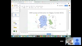
Seogi Kang leads the meeting this week. To characterize large-scale hydrological structures at Edmonton to Calgary (ECC) corridor, time-domain airborne EM data are inverted, and a conductivity model is recovered (30km x 30 km). From the obtained conductivity model, we extract important hydrogeologic information about this region such as map of potential aquifer and 3D lithology model.
A
B
B
D
C
E
C
C
C
Okay,
sorry
about
that
yeah
there's
been
I've
noticed
a
couple
things
like
that
everyone
so
now
there's
a
process
that
just
like
spins
out
of
control
and
you
just
kill
it
and
then
it's
fine
do
we
know
which
was
it
I
there's
one
called
dissed
noted
D
is
TN
o
te
D,
but
yours
is
usually
so
folks.
The
firewall
thing
no.
D
And
what
and
they
they
are
maybe
interested
in
in
that
region.
So
what
I'm
going
to
talk
about
is
the
Warren
and
ground
electromagnetic
inversion
at
the
Sylvan
Lake,
so
I
kind
of
like
starting
with
that
one
to
start
with
like
a
bit
of
motivation
here,
so
this
is
Steve.
I.
Think
that
my
background
about
this
region
is
pretty
low
right,
like
I'll
do
my
best.
So
this
is
the
Edmonton
and-
and
this
is
the
Calgary,
so
what
this
is
what
they
call
Edmonton
to
Calgary
corridor
so
EC
see.
D
C
F
D
Maybe
I
think
the
Central
Valley
is
about
that
that
so
it's
a
huge
region
and
what
this
such
the
small
patches
showing
is
a
different
types
of
airborne
e/m
survey.
So
there
are
multiple
airborne
observe
a
which
covers
this
full
whole
region,
and
the
idea
is
like
they
want
to
know
what
is
the
conductivity
structure
of
this
entire
region
and
by
by
using
conductivity?
They
want
to
have
some
sort
of
hydrogeological
information
like
where's,
the
aquifer
where's
the
aquitard.
So
but
you
cannot
really
see
that
so
in
the
ground.
D
This
is
very
holistic
view,
because
the
past
kapu
formation
is
bad,
like
it's
a
severe
unit
and
kind
of
in
details
in
past
kapu
formation,
they're,
probably
some
10
stones,
which
could
be
an
aquifer
they're,
probably
some
mud,
stone
or
clay,
which
can
be
also
not
so
I
mean
like
in
that
past
confirmation
distinguishing.
What
are
they
where
they
are?
It's
actually
an
important
goal,
and
the
region
that
we're
focusing
on
is
mostly
just
basket
to
formation.
So
we
don't
really
need
to
worry
about
other
units.
D
And,
what's
like
what
we're
seeing
with
the
electromagnetics
is
not
a
hydraulic
conductivity,
it's
an
electrical
conductivity.
They
probably
have
some
similarity,
but
they
are
a
different
property.
So
we
need
to
focus
on
what
we're
saying
in
the
electromagnetic
and
what
we
want
to
do.
As
I
said,
we
want
to
distinguish
this
two
unit
sandstones
and
not
stones.
Sandstone
usually
have
high
resistivity
and
most
on
has
slow
resistive.
So
when
we're
looking
for
an
aquifer
in
this
case,
we're
basically
looking
for
a
resistor,
so
that's
that's
the
target.
D
D
So
we
got
multiple
like
a
surveys,
but
basically
it's
a
it's
a
different
methodologies,
but
we're
seeing
same
cognitive
restructures
so
probably
potentially,
if
he,
if
you
do
a
good
job
where
we
can
well,
you
can
out
of
it,
we
can
have
a
common
cognitive
restructuring
if
not
we're
in
trouble
or
there
probably
something
we
don't
know,
and
this
is
the
Geo
temp
system.
So
this
is
the
plane
and
then
plane
flies
over
a
hundred
and
twenty
meter
above
the
surface.
And
this
so
we
have
the
transmitter
put
in
the
current
into
the
ground.
D
Like
135
meter,
far
from
from
the
transmitter
in
horizontal
direction
and
it's
fitted
about
like
70
meter
above
the
surface,
so
this
is
a
transmitter
and
that's
mystery
breath
and
that
we're
measuring
kind
of
multiple
time
Channel,
it's
not
a
single
value.
So
for
at
one
point
we
got
like
10
to
20
points,
I.
D
I
haven't
ever
got
to
the
point
where
actually
damnit
M
is
basically
no.
Never
cam
is
the
as
I
say
it's
a
ground
loop
and
then
you
have
a
one
loop
in
one
receiver
point.
So
it's
that
very
similar
to
you
can,
but
but
it's
on
the
ground,
so
it's
pretty
similar
but
probably
more
sensitive
to
the
near
surface
compared
to
210.
D
This
is
actually
quite
different
serving
so,
as
I
said
before,
we
use
the
ground
loop,
but
now
we're
using
the
electrodes
we're
actually
kind
of
grounding
those
electrode
to
the
earth
and
we're
measuring
some
electrical
signals.
So
this
is
actually
a
different
different
measurement,
but
but
we're
seeing
the
same.
Conductivity
structures
versus
Earth's
doesn't
change,
although,
where
our
methodology
is
changing
and
like
the
technique,
what
we're
using
is
an
inversion.
So
what
we're
doing
we're
measuring
electrical
signals?
But
that's
not
what
we
want.
We
want
to
know.
What
is
a
conductivity
structure
of
the
earth?
D
Look
like
so
we
need
some
sort
of
like
technique
to
to
do
so,
and
here's
a
like
bit
of
idea,
the
first
one
we
want
to
find
a
conductivity
model
to
fit
our
data,
so
we
need
to
find
the
model
m
and
then
f
is
just
our
for
modeling
operator.
So
we
know
the
physics
we
put
the
M.
We
want
to
make
sure
this
predictive
data
is
similar
enough
to
our
observed
data.
So
that's
like
very
minimal
condition
and
and
then
we
can
but
like
let's
say
we,
you
know
some
a
prior
information.
D
D
Okay,
it's
a
little
sparse,
I
kind
of
skip
this
step,
but
the
and
that
I
just
want
to
comment
that
cuz
that
we
can
kind
of
handle
each
methodology
separately
or
we
can
invert
them
together
to
obtain
a
common
conductivity
model.
So
anything
it's
just
a
little
bit
kind
of
fancy
technique,
but
it's
nothing
nothing
special!
So,
let's
get
down
to
the
main
mat
resort.
So
this
is
the
EC
resistivity
inversion.
D
So
remember
it's
about
like
a
it's
about
a
kilometer
length
from
here
to
there
at
one
point
a
so
two
kilometer
length-
and
this
is
the
recovered
conductivity
model.
So
rad
here
is
high
resistivity,
so
this
color
bar
is
in
resistivity.
So
this
is
high.
Resistivity
and
background
is
fairly
conductive.
So
remember
what
we
were
looking
for.
It
was
a
resistor
and
it's
about
like
a
meter
below
and
the
thickness
of
this
resistor
is
about
22
meter,
20
meters.
D
So
that's
actually
a
good
imaged
and
let's
move
on
so
we
got
another
ground
survey
called
nano
can
remember
the
surface
loop
and
the
single
receiver.
So
what
we're
doing
before?
We
actually
were
working
on
a
2d
the
main,
but
here
what
we're
going
to
do
a
1d,
so
we're
going
to
assume
the
later
structure.
The
earth
structure
is
basically
one
V
and
then
so
each
point
at
each
kind
of
source
and
receiver
point
we're
going
to
have
a
one
these
structures.
D
So
this
is
actually
a
1d
structure
at
this
point
and
that
point
and
that
point
and
that
point
so
can
definitely
see
some
resistor
at
the
near
surface,
about
10
meter
below
and
thickness
about,
20
meter
ish
and
you
can
see
on
the
other
line,
which
is
green
and
a
similar
structures.
And
if
you
compare
that
with
the
DC
resistivity,
it's
actually
similar.
So
let's
look
at
here:
we've
got
a
resistor
here.
Is
a
destroyer
here,
resist
RIA
and
that
we
have
a
very
weak
resistor
at
this
point
and
that's
actually
what
it
is.
D
So
let's
do
a
little
bit
more
kind
of
serious
comparison,
so
I'm
going
to
pick
a
point
here
and
the
vertical
profile
of
the
DC
resistivity
and
compared
with
the
Nano
tap
and
that's
how
it
looks
like
it's
not
exact,
but
there
are
actually
consistent
but
consistently
seeing
this
resistor
and
the
conductive
background
and
same
as
here.
So
that's
actually,
that's
actually
good
right.
E
D
River
leaves
in
two
different
methodology
and
we're
seeing
similar
conductivity
structure.
That
really
adds.
Oh,
okay,
there's
something
there's
something
going
on
and
we're
getting
a
consistent
reserve,
which
is
actually
a
good
it's
sign,
and
that
was
the
ground
bronze
early.
But
what
step
autumn
leg
of
the
ground
survey?
It's
actually
hard.
You
need
to
go
there.
You
need
to
like
lay
out
the
loop
or
you
need
to
like
put
the
electrodes
into
the
ground
and
even
just
doing
a
kilometer
survey.
D
D
It's
like
you
can
you
can
fly
over
that
region
pretty
fast
and
if
you
can
recover
pretty
pretty
much
like
the
same
quality
of
the
conductivity
structure
with
with
the
ground
survey?
That's
actually
that's
actually
great!
So
that's
that's
our
motivation
and
we're
going
to
move
on
to
our
born
data.
As
I
said,
because
we
got
some
motivation
and
at
this
region
we
got
about
10,000
something
locations
I,
just
on
some
of
the
other
out
there
more
if
it's
probably
a
hundred
thousand,
if
I
didn't
down
sample
it's
about
hundred
thousand.
D
G
D
That
point
and
invert
them
and
compare
with
the
ground
ground
ground
measurements,
because
why
we
want
to
see
the
similarity
the
same
as
like,
as
we
seen
in
between
the
sea
and
the
nano
time.
So,
if
I,
just
starting
with
the
data
as
an
anthem
data
at
black
star
that
looks
like
this
and
the
red
star
looks
like
that,
so
that's
north
and
south,
and
you
can
north
black
and
south
red.
So
those
are
the
day
again.
So
by
looking
at
the
data,
we
don't
have
that
much
idea
how
the
earth
looks
like.
D
So
that's
why
we
need
to
do
an
inversion
and
here's
the
inversion
reserve
member
at
the
mallet
m1,
the
red
one,
definitely
see
the
resistor
at
the
new
surface
and
the
the
black
one
doesn't
show
and
how
about
the
two
of
them
red
one
actually
show
some
resistor
not
as
like
high
resolution,
as
now
that
I'm
at
the
very
near
surface.
But
still
it
is
showing
that
and
that's
actually
expected
because
the
geochemist
much
less
resolution
at
the
very
near
surface
compared
to
nab
them
think
about.
D
On
the
ground,
it's
much
more
sensitive
compared
to
airborne
search,
so
you
can
better
resolve
that
new
surface
and
also
black
we're
basically
seeing
sort
of
background
the
in
as
a
first
order
it's
actually
matching,
but
we
can
go
a
little
bit
more
as
I
said,
rather
than
inverting
them
separately.
We
can
invert
them
together,
see
if
we
can
actually
fit
the
data
with
a
common
conductivity
model.
D
So
if
I,
that's
actually
what
we
call
joint.
So
if
we
actually
invert
these
two
dataset
together
and
that's
the
common
conductivity
model,
so
we're
fitting
both
theta-
and
this
is
the
recovered
conductivity.
So
we're
actually
getting
better
resolution
at
the
near
surface
because
of
the
nano
time
and
we're
also
seeing
a
little
conductor
at
the
deeper
part
better
for
his
wordplay.
That's
actually
helping
right
we're
getting
a
near
surface
conductivity
better.
We
probably.
D
See
the
deeper
part
as
well,
so
it's
actually
kind
of
nice
anyway.
Here
the
point
is
actually
geo
cam
with
the
geo
10,
we
can
recover
kind
of
pretty
good
quality
of
the
conductivity
model.
Okay,
so,
let's
now
kind
of
search
act,
all
the
locations
we
actually
handled
to
location
because
we
go
actually
10,000
location,
let's
invert,
all
of
them
and
see
what
we
can
actually
get
out
of
it.
D
E
D
D
Anyway,
so
that
Sylvan
Lake
is
about
here,
this
is
a
topography.
So
the
large
like
this
brown
color
means
high
to
poverty
and
the
blue
is
low
topography
and
that's
the
7
Lake
and
what
I
did
actually
I
inverted
all
of
those
10,000
sounding
location,
and
this
is
actually
a
basically
one,
the
inversion
and
then
I'm
inverting,
all
of
them
together,
but
still
on
what
I'm
getting
is
the
1d
structure,
but
the
just
for
a
visualization
purpose,
I
kind
of
interpolate
that
back
to
in
3d.
D
So
this
is
what
I'm
showing
so
that's
actually
a
3d
model
and
that
planned
view.
It's
about
I
think
it's
at
very
near
surface.
So
this
was
the
DC
line.
Do
you
remember
love
with
where
we
compared
the
conductivity
structure
and
if
I
actually
see
this
profile
at
dotted
line?
That
looks
like
that
and
you
can
see
other
profile
another
profile,
so
we're
basically
seeing
kind
of
near
surface,
resistor
and
I
think
this
high
resistor
may
have
probably
high
potential
to
be
to
be
an
aqua
good.
D
I
prefer
I,
guess
so,
and
then
you
can
see
a
conductor
below.
So
those
are
the
like
kind
of
similar
structure
that
we're
seeing,
but
at
this
full
region
and
what
we
could
do.
Okay,
so
that's
what
we've
got
and
we
can
see
some
resistors
and
conductors
potentially
an
aquifer
or
or
or
lack
so,
let's
actually
just
simply
make
it
cut
off.
So
we're
going
to
go
I'm
going
to
pick
some
sort
of
resistivity
value
high
enough,
maybe
around
twenty
five
or
thirty,
and
then
this
like
region.
D
This
volume
will
be
a
high
resistor
I,
resist
it
like
something.
A
volume
having
high
resistivity
and
I
can
consider
that
as
an
aquifer,
for
instance,
as
a
very
simple
matter,
and
that's
aquifer
happening
about
ten
meter
depth
and
how
about
the
awkward
part,
I
could
actually
do
a
same
sort
of
procedure.
Okay,
I'm
going
to
cut
off
like
I'm,
not
I,
don't
I,
don't
care
about
the
hyde
resistivity
volume.
I'm
gonna
pick
that
very
low
having
volume
having
low
resistivity
and
that's
the
clay.
And
here
it's
a
this
scale
is
exaggerated.
D
D
Think,
okay,
you
can
finish
there,
but
they
I
was
kind
of
curious
depends
upon
now
that
was
sort
of
the
geophysics
alright
and
but
like
this
is
not
the
end
of
the
story.
So
as
a
geophysicist,
you
need
to
transfer
this
information
to
different
groups
of
people
who
may
be
really
interested.
So,
for
instance,
say
you
can
you
can
provide
an
information
from
somebody
who
wants
to
do
a
run
water
exploration,
for
instance,
or
hydrogeologist?
Who
wants
to
do
some
sort
of
flu
simulation
to
predict?
What's
going
to
happen
in
this
area?
D
So
there
are
multiple
like
groups
of
people
who
might
be
a
user
for
this
research,
so
I'm,
just
kind
of
like
making
in
it
like
a
hypothesis
and
I,
want
to
show
how
we
can
provide
kind
of
relevant
information
from
for
those
different
audiences,
and
the
first
like
the
first
case
was
considering
was
for,
let's
say
somebody
who
wanted
to
do
a
groundwater
exploration,
so
they
want
to
know.
Okay,
where
do
I
want
to
drill?
Okay,
so
say,
and
this
is
actually
an
interesting
plot.
This
is
the
recovery
resistivity.
D
D
So
that's
what
that
that's,
what
we're
doing
so,
what
I'm
doing
I'm
using
some
sort
of
like
clustering
technique
so
remember
like
a
whole
bunch
of
different
vertical
profile,
I
want
to
classify
that
as
a
four
different
units.
So
so
those
are.
The
representative,
like
four
different
representative
from
my
whole,
soundings
10,000
soundings.
So
I
got
c1,
c2,
c3
and
c4
okay,
so
let's
consider
two
c1
and
then
all
those
soundings
or
the
vertical
profile
or
resistivity
profile
kind
of
included
in
the
see
one
that
looks
like
this,
you
can
definitely
see
okay.
D
D
That
many
things
that
much
things
like
we
don't
really
see
a
big
resistor
if
that's
c1
and
c2.
This
is
probably
an
interesting
one
for
us,
so
it's
kind
of
similar
right.
It
can
definitely
see
that
this
could
be
a
good
representative
of
all
of
this
vertical
profile
and
that
you
can
definitely
see
big
resistor
at
the
near
surface
and
that's
potentially.
What
we're
interested
is
that
this
structure
is
actually
interested
as
an
aquifer.
D
How
about
c3
it's
actually
a
little
bit
kind
of
arguable.
Is
that
a
good
representative?
Well,
so
that's
actually
that's
where
you
can
see
the
covariance.
So
if
you
have
a
local
variants,
that
means
most
of
the
profile
is
actually
pretty
simple,
but
if
you
have
a
high
covariance
yeah,
it's
a
bit
arguable
and
how.
D
It
may
not
quite
be
the
case
that
were
we're
looking
for
or
I
think
they're,
probably
something
something
going
on,
and
then
that's
where
ever
our
assumptions
it's
not
valid
or
we
have
the
high
noise
or
something
like
that.
So
I
think
that's
potentially
what
those
c3
and
c4,
but
let's
not
worry
about
c3
and
c4,
let's
focus
on
c1
and
c2,
where
we
actually,
that
can
really
consist
on
1d
structures.
D
So
c1
we
actually,
if
you
focus
on
that,
we
got
near-surface
resistor
and
that
could
be
a
potential
aquifer
and
we
see
that
the
little
bit
deeper
conductor
see
there's
like
well
there's
a
little
bit,
but
basically
there's
no
near
surface
resistor,
but
we
can
see
the
dip
conductor.
So
those
are
two
very
distinct
and
dominant
unit
at
this
region,
and
we
could
do
a
little
bit
of
analysis
about
c3
and
c4.
What
could
be
like
what's
happening
there?
So
I'm
just
plotting
up
the
topography?
D
Okay-
and
also
this
dotted
line-
shows
where
you
have
big
power
line
effect.
So
in
the
data
you
can
actually,
they
usually
monitor
the
power
line
effects.
So
you
can
pick
some
sort
of
threshold
and
see
where
you
have
a
high
power
line
effects,
because
that's
basically
the
noise-
and
it's
actually
like
look
at
here,
so
we're
picking
up
this
high
topography
and
that's
where
we're
seeing
either
c3
and
c4.
D
So
we
were
pretty
sure
okay,
this
is
where
our
assumption
is
not
valid,
so
we're
seeing
some
sort
of
odd
strata,
so
he
may
you
may
not
want
to
leave
that
structure
is
actually
correct,
so
this
is
sort
of
like
a
kind
of
checking
where
your
assumption
is
okay,
Mashable
and
also
about
this
location.
You
got
like
high
quality,
so
we're
picking
that
up
and
our
line
noise
may
be
here.
An
Oscar
are
about
the
power
line.
Where
is
it?
It's
attribute?
Pretty
hard
to
see
the
good
correlation,
so
maybe
power
line
noise.
D
It's
not
a
like
we're
know.
It's
not
really
making
a
big
big
impact
to
to
this
data
sets
I
guess
anyway.
So
it's
a
it's
a
it's
a
kind
of
away.
So
what
I'm
going
to
do?
I'm
gonna
ignore
all
the
seat,
like
all
the
information
from
c3
and
c4
I'm,
going
to
focus
and
see
you
on
the
c2,
so
C
3
and
C
4
is
in
Goa
following
process.
D
C
F
D
F
D
E
A
D
A
A
D
And
I
think
that
what
a
here
don't
be
confused,
cuz
yeah
I'm,
not
ignoring
all
of
this
location,
so
I'm,
just
cherry
picking
a
couple
of
location
which
has
been
odds,
I,
think
that
what
I'm
actually
removing
it's.
Just
probably
this
point
like
big
outliers,
have
a
big,
resistor
and
I
think
we're
we're,
making
an
assumption,
Oh
our
structures
really
smooth
them
and
1d.
That's
I
think
in
dev
assumption.
D
Okay,
so
it'll
be
complicated,
but
I
think
this
is
probably
what
I
don't
know
if
somebody
wants
to
okay
we're
going
on
to
drill
and
here's
probably
my
my
answer.
Okay,
please
just
be
spot
that
arrow
board
data.
If
that's
given
so
I
remember
we
did
the
like.
If
you
find
the
two
coasters
right,
one
was
see
one
showing
a
big
resistor
at
the
near
surface
and
see
two.
D
Like
kind
of
berries
shot
like
a
kind
of
weak
resistor
at
than
their
surface,
and
if
I'm
at
that
app
on
a
2d
plane
right
so
Radley's
see
one
and
the
blue.
You
see
two
so
rad
I
think
this
is
where
you
got
pretty
big
potential
to
find
that
find
an
aquifer.
I
guess
compared
to
c1,
so
I
think
that's
pretty
useful,
useful
map.
D
D
E
D
It's
actually
matching
right,
braum
measurement
and
then
information
from
airborne
data.
It's
actually
magic.
It's
actually
a
good
sign
and
here's
another
thing.
While
we
good
to
know
we
know
like
most
of
the
resistor
happening
up
top
50
meters,
so
let's
actually
take
the
all
these
kind
of
layers
included
in
the
top
50
meters
or
we
go
and
then
what
we
care
is
actually
resistivity
thickness
product,
but
you
recall
resistance.
So
that's
actually
what
you
can
tell
right.
D
We
have
a
lot
of
non
uniqueness
about
the
thickness,
but
I
mean
this
is
actually
a
pretty
good
information.
So
what
I'm
going
to
do?
I'm
gonna
sum
the
product
have
resisted
the
thickness
up
to
n.
So
it's
about
50,
meter
and
I'm
gonna
plot
that
value
on
the
2d
plane,
so
high
high
resistivity
high
resistant
means
you
probably
have
higher
potential
to
find
an
aquifer.
A
D
Guess
so
I
think
if
you
go
back
and
forth,
it's
basically
that
they
have
nicely
about
those
clusters
right,
C,
1
and
C
2,
but
in
C
2
we
can
actually
show
oh,
where,
where
we
got
even
more
possibility
to
find
an
aquifer,
so
I
mean
it's
not
hard,
but
I
think
it's
probably
a
good
and
useful
information.
If
you
don't
have
that
much
information
region
and
I,
think
that
was
a
lift
for
the
kind
of
sort
of
ground
exploration.
Point
of
view.
D
Now,
how
about
like
hydrogeologists,
who
want
to
have
a
large-scale
lithology
model,
to
file
to
kind
of
proceed
there
for
simulation,
so
what
they
usually
do?
They
probably
have
some
wells
and
then
you
have
some
Recology
information.
They
interpolate
fly
from
very
sparse
point
to
a
large
area
and
then
proceed
there
through
simulation.
So
hope
that
means
there
are
a
lot
of
uncertainties
in
and
in
their
model.
So
how
can
we
help
them
to
to
proceed
kind
of
better
quality,
high
quality
simulation,
so
here's
a
one
other
way
so
we're
basically
using
the
same
technique.
D
I,
what's
called
like
a
Gaussian
mixture
and
what
we're
doing
is
basically,
it's
actually
been
simple,
we're
doing,
1d
clustering,
so
let's
say
we're
putting
just
a
continuity
value
and
find
some
sub
clusters,
and
then
we
did
the
same
process.
You
find
three
clusters
what
we
call
r1,
r2
and
r3.
So
that's
our
effect
with
the
Gaussian
mixture.
So
this
is
a
histogram
and
r1
is
about
15,
which
is
about
the
background
and
that's
the
gray
and
r2
is
till
12.
D
Its
conductive
r3
is
a
resistor
up
top
and
that's
where
we
got
the
DC
line,
see
the
big
resistor
like
a
thick
thicker,
resistor
and
the
shallower
so
I
mean
it
said
it
says
it's
not
like
a
very
fancy
way,
but
I
mean
it
with
considering
you
don't
have
that
much
information,
if
you,
if
you're
just
given
the
airborne
beta.
This
is
probably
what
you
could
think
that
was
yeah
I
still
have
a
bit
of
challenges
and
I'm
like
sort
of
like
well
technically
I.
D
Don't
have
any
she'll
understand
just
like
having
some
challenges
to
dig
up
information
about
this
region.
It
seems
like
that
there
are
a
lot
of
like
a
lot
of
worlds
tons
of
wells,
and
actually
they
worked
a
lot
at
this
region,
I
think
but
you're,
one
at
the
end
like
Ron
right.
Everyone
here
was
very
small
part
I
mean
they
actually
a
lot
of
war,
but
I
was
actually
when
I
was
kind
of
doing
a
literature
review.
It
seems
like
the
airborne
I
ended.
D
It
wasn't
in,
like
it
wasn't
in
their
process
to
build
up
the
model,
so
basically
I
think
how
they
are
ended
up
using
was
gamma
ray
lock,
and
that
was
it
I
mean
and
then
and
the
following
information.
They
got
from
the
core
samples
with
that
I
mean
they're,
basically
kind
of
interpolating
to
like
everywhere,
using
some
to
you
statistics
and
that's
something
that
I'm
not
sure
how
how
how
this
information
can
be
sort
of
like
sneaking
into
their
process
and
provide
some
useful
information.
D
D
D
C
A
E
A
D
A
D
E
D
So
here,
I
like
a
this,
is
fairly
conductive
region,
and
so
actually
water
itself
doesn't
make
that
much
far
outside.
That's
something
that
I
wasn't
sure.
Okay,
so
it
doesn't
necessary,
mean
like
it's
a
resistor,
but
it
doesn't.
This
thing
mean
that
that
it
actually
includes
the
water
or
not
so
we're
actually
like
here.