►
From YouTube: IETF104-ICCRG-20190328-1610
Description
ICCRG meeting session at IETF104
2019/03/28 1610
https://datatracker.ietf.org/meeting/104/proceedings/
A
That
was
super
deliberate.
Nobody
will
awake.
Let's
get
started,
it's
not
just
my
Mike
Brian,
all
right
I'm,
not
repeating
Brian's
comments
to
the
mic,
but
let's
get
started.
This
is
IC
c
RG.
If
you
don't
care
much
about
condition
control,
you
are
in
exactly
the
right
room.
You
might
learn
a
few
things.
A
A
A
A
A
A
Thank
you,
sir
who's
I
heard
a
voice.
I
can
see
yes
Brian.
Thank
you.
Thank
you.
Thank
you.
Thank
you.
Moving
on,
we
have.
We
have
a
packed
agenda
today
we
have
only
four
presentations,
but
all
four
of
them
interesting
talks,
and
so
there's
a
fair
bit
of
time
for
each
one,
I'm
going
to
be
I'm,
gonna,
try
and
stick
to
the
time
that
I
have
written
out
there
and,
as
always,
you
will
all
go
past
the
time
so
we'll
see
how
this
goes.
A
B
So
I'm
going
to
be
talking
about
bbr
v2,
which
we
think
of
as
a
model
based
congestion
control.
This
is
joint
work
with
my
colleagues
at
Google,
you
chung
Sohail,
ianvictoria
Rajan,
you
suck
Matt
and
Van
Jacobson
next
slide.
Please
so
I'm
gonna
focus
on
the
be
BRB
to
research,
update,
I'm,
talking
about
improvements
between
VBR,
v1
and
v2.
B
B
B
Bb,
everyone
was
Ross
agnostic
which,
in
certain
scenarios
with
Banach
buffers
or
a
QMS,
keeping
the
queue
at
1.5
be
Peters
shorter.
That
could
result
in
high
packet
loss
rates
via
v1
was
easy
on
agnostic
as
well.
Did
not
use
CCN
signals
and
with
the
initial
release
there
could
be
low
throughput
for
paths
with
high
degree
of
data
or
AK
aggregation,
and
here
the
the
biggest
issues
you
would
see
with
Wi-Fi
paths,
with
no
our
TTS
say
one
to
ten
milliseconds
and
then
another
issue
with
me.
B
One
was
that
there
could
be
pretty
severe
throughput
variation
due
to
quite
low
ceilings
in
when,
in
a
small
period
of
time
that
they're
in
probe
RT
t
mode,
then
with
BB
r
v2.
We
were
trying
to
tackle
all
of
these
issues
and
I'll
give
some
examples
of
the
design
changes
in
the
resulting
behavior.
So
for
coexistence
with
reno
in
cubic.
B
So
here's
a
scenario
with
a
15
megabit
bottom
link,
a
40
milliseconds
rip
time,
one
VDP
a
buffer
for
cubic
flows,
one
PBR
be
to
flow,
and
you
can
see
the
the
BP
RV
to
flow
is
is
playing
along
nicely
there
at
the
bottom,
in
the
pink,
achieving
an
approximately
fair
share.
The
reasonably
low
retransmitted
rate
matching
cubics
here.
B
So
the
next
major
improvement
is,
is
using
packet
loss
as
an
explicit
signal
with
an
approach
that
sort
of
has
an
explicit
target
loss
rate
ceiling,
which
I'll
talk
a
bit
about
a
bit
about
later.
On
this,
we
also
talked
about
it,
ITF
102
and
here's
a
quick
scenario
just
to
sort
of
illustrate
the
behavior
with
this
algorithm.
So
here
we
have
six
VP
of
the
two
flows
in
a
very
shallow
buffer.
B
That's
only
5%
of
the
BDP,
only
49
packets,
but
the
flows
start
staggered
and
achieve
an
approximately
fair
share
and
with
the
reason
being
we
transmit
rate,
given
how
shallow
the
buffers
so
be
BRB
to
uses
ECN
as
a
signal
now
DC
TCP
style
ecn.
If
it's
available
to
help
keep
the
queues
short
and
to
illustrate
the
kind
of
behavior
we're
talking
about
here,
we
have
20bb
our
v2
flows,
starting
staggered
every
100
milliseconds,
it's
a
1
gigabit
bottleneck
link
in
a
1
millisecond
round
trip
time.
The
ECM
marks
here
are
from
the
linux.
B
Coddled
queue
disk
with
the
default
settings,
except
for
the
c
e
marking
threshold
at
242
microseconds,
which
is
about
20
pounds
worth
of
queue.
Okay,
we
have
0
retransmits,
pretty
decent
fairness
and
our
TTS
are
fairly
low.
The
median
OTT
is
right
around
the
marking,
the
threshold
and
the
rest
are
reasonably
well
controlled.
B
So
there
are
also
improvements
for
high
throughput
for
paths
with
large
SKUs
of
aggregation,
notably
as
I
said
Wi-Fi,
and
to
achieve
that
v2
explicitly
estimates.
The
degree
of
aggregation
that
had
seen
recently
and
now,
maybe
in
the
data
path
and
maybe
in
the
act
path
either
way.
The
aggregation
shows
up
in
the
extreme
and
bbr
tries
to
characterize
that,
and
we
talked
about
the
details
of
that
it
ITF
101.
B
Last
March,
you
can
find
the
slides
there
on
YouTube
we're
seeing
be
BRB
to
match
Kubek
throughput
for
users,
specifically
on
Wi-Fi
links
and
overall
and
in
control
tests
for
seeing
reasonable
behavior.
You
can
see
here
on.
The
right
is
a
time
sequence
plot
of
a
be
BRB
to
transfer
to
my
laptop
at
home.
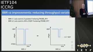
B
The
final
major
design
change
is
to
reduce
the
throughput
variation.
So
when
BB
everyone,
if
you
had
to
enter
probe
itt,
perhaps
because
it
was
a
bulk
flow,
that's
been
going
more
than
10
seconds
or
so
bbr
v1
would
cut
the
seal
into
4
packets
in
v2.
You
know
we
can
cut
the
c1
to
50%
of
the
bdp
to
still
achieve
reasonable
throughput,
even
while
attempting
to
probe
the
the
to
a
propagation
delay.
B
So
those
are
the
major
improvements
in
v2.
As
a
quick
summary,
you
can
sort
of
consider
how
B
to
lines
up
with
v1
and
cubic
as
I
said,
the
it's
a
model
based
congestion
control
and
here
specifically
the
model
parameters
that
we
feed
into
the
state
machine
for
BB.
Are
we
to
include
the
throughput,
the
RTT
or
men,
ou
TT,
the
max
degree
of
aggregation
we've
seen
recently
in
the
max
amount
of
data?
We
think
it's
reasonable
to
keep
in
flight
and,
as
I
said
BB.
B
Our
v2
has
this
sort
of
explicit
loss
rate
target
and
an
explicit
response
to
congestion
to
eat,
DC,
TCP
style
congestion
and
the
startup.
Not
surprisingly,
has
a
sort
of
slow
start
style,
behavior
of
doubling
the
throughput
until
we
see
the
either
the
throughput
plateau
or
the
ecn
or
loss
rate
exceed
the
design
parameter
or
threshold.
B
B
We're
gonna
update
the
BB
our
internet
drafts
to
reflect
the
latest
vb
r
v2
code,
because
I
know
there
are
people
out
there
that
are
interested
in
working
with
the
algorithm
based
on
the
draft
rather
than
the
code.
I
would
note
that
the
code
we
try
to
we,
we
have
made
a
dual
BSD
GPL,
so
hopefully
folks
in
the
BSD
ecosystem
can
use
it,
as
is
if,
if
they
are
interested,
but
that
ain't
right
so
I'm
gonna
try
to
do
a
lightning
over
year.
C
D
B
So,
just
a
quick
I
mean
you're
gonna
try
to
do
a
lightning
overview,
the
BRB
to
design
many
of
these
slides.
We've
shown
a
previous
IETF,
so
I
just
thought
it
would
be
useful,
have
a
quick
overview
all
in
one
spot.
For
so
at
a
10,000
foot
view
you
can
think
of
the
design
as
basically
consisting
of
a
system
that
takes
as
inputs,
measurements
from
the
network
traffic
that
it's
controlling
and
it's
looking
at
a
couple,
different
signals
to
the
throughput
or
delivery
rate.
B
The
delay,
that
is,
the
RTT
delay,
the
loss,
events,
ecn
mark
events
and
those
are
all
fed
into
a
network
path
model
inside
PBR.
And
then
the
parameters
of
the
network
path
model
are
used
to
control
the
evolution
of
the
state
inside
the
state
machine
inside
PBR,
and
then
that
in
turn
makes
adjustments
in
the
output
parameters,
which
are
the
rate
which
you
can
think
of
as
a
sort
of
pacing
rate
for
the
sending
process.
B
Until
it
has
a
maximum
amount
of
data
or
or
until
pacing
says
you
can't
set
any
more
right
now.
So
so
that's
a
the
big
picture.
If
we
look
at
the
drill
down
into
the
model
and
what's
inside
the
model,
you
can
sort
of
visualize
it,
as
is
depicted
here
in
the
diagram.
That's
a
time
sequence
diagram
with
a
sequence
on
the
y-axis
time
on
the
x-axis,
the
green
is
showing
send
events.
The
acts
are
showing
up
as
blue
here
here.
B
I've
drawn
them
is
as
pretty
bursty
acts
because
that
these
days,
that's
a
pretty
pretty
typical
behavior,
whether
it's
high
speed,
8
Ethernet,
Wi-Fi,
cellular
DOCSIS.
They
all
have
aggregation
pretty
significant
levels
and
you
can
sort
of
visualize
each
of
the
parameters
here.
The
first
one
is
the
maximum
bandwidth
that's
available
recently
to
this
flow,
the
second
one
you
can
think
of
as
the
min
RTT
seeing
recently,
which
serves
as
an
estimate
of
the
tumor
propagation
delay.
Then
there's
the
maximum
amount
of
inflator
that
we
think
is
reasonable.
B
That's
reasonable
to
keep
maximum
amount
of
data
it's
reasonable
to
keep
in
flight
so
because
of
that
BB
r
v2
maintains
both
a
short-term
bandwidth
and
in-flight
estimate
and
a
long-term
bandwidth
and
in-flight
estimate,
and
you
can
think
of
this
as
sort
of
being
analogous
to
cubic,
which
has
a
sort
of
short
term
SS,
thrush
estimate
and
then
a
longer
term
W
max
value.
That's
a
higher
amount
of
in-flight
data
that
it's
hoping
to
quickly
progress
back
up
to
you
with.
If
everything
goes
well,
it's
sort
of
analogous
to
that.
B
So
a
high
level.
The
adaptation
of
the
model
basically
estimates
that
then,
with
an
in-flight
2d
set
of
parameters
over
both
the
short
term
in
the
long
term,
with
the
goals
being
not
surprisingly,
a
high
throughput
and
for
bbr
importantly,
we're
trying
to
be
able
to
maintain
that,
even
when
experiencing
some
moderate,
particularly
amount
of
random
packet
loss
and
then
we're,
of
course,
trying
to
keep
low
queue
pressure
and
the
basic
approach
here
is
sort
of
twofold.
B
An
in-flight
estimate
tuple
that
basically
bounds
the
behavior
using
the
latest
delivery
process
and
Lawson
ECM
signals
that
we're
seeing
and
the
intuition
here
is
basically,
what's
the
bandwidth
and
in-flight
delivery
process
that
we're
seeing
right
now
and
we're
seeing
you
see
any
lost
signals,
that's
an
indication
that
we
need
to
adapt
quickly
to
those
signals
that
we're
seeing
right
now
to
maintain
reasonable
queuing
levels.
And
then
the
second
part
of
this
picture
is
that,
of
course,
periodically.
B
B
That's
the
basic
high-level
picture
of
the
model
so
to
consider
the
details
of
how
it
evolves,
I
think
it's
useful
to
consider
a
more
concrete
example.
So
it's
an
interesting
question:
how
do
we
adapt
to
a
packet
loss
signal
given
the
ambiguities
involved?
So
if
we
consider
this
this
example,
we
hear
we
have
a
shallow
buffered,
high-speed
wind
would
say:
100
millisecond,
round-trip
time
and
app
does
occasional,
200
mm
packet
writes.
These
are
RPC
requests.
Rpc
replies.
B
Web
object
replies,
something
like
that
and
let's
consider
a
case
where
the
available
bandwidth
drops
from
something
really
high,
say:
12
gigabits
per
second
down
to
12
megabits
per
second,
which
is
from
a
thousand
packets
per
millisecond.
On
a
one
packet
or
a
millisecond
and
of
course,
that's
a
big
drop
so
in
the
first
right
after
that
bandwidth
drops,
if
we're
continuing
at
the
same
rate,
there
will
likely
be
very
high
packet
loss
and
there's
an
interesting
idea,
though,
about
the
low
delivery
rate
that
we
see
there
of
two
packets
in
their
own
trip
time.
B
It
was
a
question
of
to
what
extent
is
that,
due
to
with
the
lack
of
data
that
was
sent
to
extent,
it
was
due
to
bursty
traffic
that
may
have
caused
that
loss
or
or
it
could
be,
a
sustained
reduction
in
the
bandwidth
available
to
that
flow.
So
the
question
is:
how
do
we?
What
do
we
do
there?
So
the
philosophy
here
the
design
philosophy
here-
is
that
to
fully
utilize
bottlenecks
of
all
kinds,
including
the
bottlenecks
with
shallow
buffers,
we
want
to
adapt
both
the
maximum
sending
rate
and
the
maximum
in-flight
meal
ow.
B
B
So
the
idea
here
is
that
if,
if
this
last
pattern
or
something
like
it
continues
repeatedly,
we
basically
want
to
gradually
reduce
the
sending
way
down
to
match
the
available
bandwidth
and
to
try
to
converge
to
an
in-flight
that
matches
the
BGP
so
that
we
can
send
the
entire
response
without
anything
being
dropped.
That's
the
the
basic
motivating
idea.
So
what
does
the
algorithm
look
like
for
the
short
term
model
adaptation?
B
Basically,
this
this
strategy
at
a
high
level
is
to
gradually
adapt,
as
I
said,
to
to
measure
delivery
process,
which
includes
both
the
bandwidth
and
the
volume
of
data,
and
this
adaptation
applies
generally,
whether
we're
in
fast
recovery,
RTO
recovery,
not
in
recovery
at
all,
whether
application,
limited
or
not,
and
the
basic
idea
is
to
maintain
a
very
recent
estimate
of
the
delivery
process,
both
the
rate
and
the
volume
of
data
and
then
upon
in
once
per
round
trip
time,
make
an
adjustment
in
those
two
model
parameters.
That
is
a
multiplicative
cut
by
30%.
B
Someone
like
cubic
except
the
the
twist
here
is
that
we
try
not
to
cut
the
model
parameters
below
the
most
recently
observed
delivery
process
values
so
that
we
try
not
to
overreact
and
try
to
match
the
recent
or
converged
on
to
in
the
recent
delivery
process.
So
that's
a
basic
idea,
so
if
we
so
that's
the
the
model
and
how
that
evolves,
if
we
switch
over
to
the
state
machine
at
a
higher
level,
the
state
machine
is
quite
similar
to
the
v1
we're
alternating,
essentially
between
probing
for
bandwidth
and
round-trip
time.
B
When
the
connection
is
warming
up,
we
have
a
startup
phase.
It's
a
lot
like
slow
start
once
the
path
we
think
is
full.
We
try
to
drain
the
queue,
and
then
we
alternate
between
probing
for
bandwidth
and
program
for
round-trip
time
so
just
to
quickly
go
through
an
example,
life
cycle
of
a
a
B
B
RB
flow
here
I'll
try
to
highlight
an
in
bold,
the
stuff,
that's
new
and
v2
versus
v1,
and
this
order
this
may
seem
similar.
B
If
you
recall
the
presentation
from
last
July,
but
I
thought
it
would
be
useful
just
to
run
through
it
quickly
again,
so
a
flow
starts
out
in
start-up
which,
like
the
traditional,
slow,
start
phase,
we're
trying
to
rapidly
discover
the
available
bandwidth
by
doubling
the
sending
radio
from
a
trip
time.
Until
we
see
that
it
looks
like
the
path
is
full.
Neither
because
bandwidth
samples
are
plateauing
or
the
loss
or
ecn
mark
rate
becomes
too
high.
B
Then
we
try
to
spend
most
of
our
time
in
a
phase
that
you
can
think
of
as
sort
of
a
cruising
where
we're
trying
to
maintain
a
low
in-flight
and
adapting
continuously
every
round-trip
time
to
whatever
loss
and
ecn
signals
that
we
see
based
on
the
algorithm
I
just
described,
and
then
when
we
decide
it's
time
to
probe
for
bandwidth.
First,
we
try
to
refill
the
the
pipe
by
sending
out
exactly
the
estimated
bandwidth.
E
B
A
shallow
buffer,
they
were
dealing
with
or
a
deep
one,
so
we
started
all
cautiously
with
a
one
extra
packet
in
flight
and
then
progressed
to
exponentially
higher
amounts
as
we
were
able
to
grow
and
fly
without
causing
the
ECM
mark
rate
or
the
loss
rate
to
go
above
the
design,
SLO
thresholds.
And
then
once
we
do
see
some
indication
that
we
filled
the
path
either
because
we
were
able
to.
We
apparently
created
a
queue
by
having
in-flight
reach,
some
multiple
of
the
BDP
or
we
hit
ecn
or
less
signals.
B
B
So
reno
has
this
sort
of
familiar
sawtooth
pattern
with
putting
an
additional
packet
in-flight
every
round-trip
time
until
the
experience
is
any
packet
loss
at
all
and
that
responds
to
a
me,
a
level
of
packet
loss
at
all
means
it
has
sort
of
a
brittle
loss
response,
because
the
c1
increases
are
linear,
one
packet
per
round
trip
time.
It
needs
a
long
time
to
fill
a
pipe,
so
it
needs
a
thousand
times
more
time
to
reach
a
thousand
times
higher
bandwidth,
which
means,
for
example,
to
fill
a
10
gigabit
hundred
millisecond
path.
B
You
mean
more
than
an
hour
between
any
sort
of
packet
loss
at
all,
which
means
you
need
a
very,
very
little
packet
loss
rate
of
two
times
10
to
the
minus
10,
which
is
not
really
achievable
in
practice.
So
people
came
up
with
cubic,
which
has
a
more
scalable
growth
curve
using
a
cubic
in
cruise
function,
but
it's
still
not
as
scalable
as
we'd
like,
so
you
still
need.
B
The
idea
here
is
that
we
try
to
have
a
scalable
exponential
growth
so
that
you
can
utilize
nearly
available
bandwidth
in
logarithmic
time
and
you
because
of
the
last
times
you
can
fully
utilize
a
in
a
big
beauty
piece
that,
even
with
a
certain
amount
of
loss
in
every
round
determined
by
the
design
parameter,
that's
the
lost
Thresh,
and
this
is
a
picture
of
a
shallow
buffer,
a
case
where
we
do
run
into
packet
loss.
If
there
is
a
deeper
buffer,
then
we
wouldn't
even
be
running
into
that
Pecola's.
B
So
quick
status
overview,
the
BRB
one
is
running
for
most
traffic
on
Google
and
YouTube
and
backbone,
but
we
are
experimenting
aprv
on
YouTube.
There
there's
some
links
there
to
other
documents
that
we've
talked
about
before
and,
in
conclusion,
were
actively
focused
on
PBR
v2
and
making
improvements
there,
including
reducing
pressure.
Improving
coexistence
with
you
know
in
cubic
there's
also
work
going
on
on
bbr
for
FreeBSD
TCP
at
the
Netflix
or
in
close
communication
with
their
excellent
team
and,
as
always,
we're
happy
to
see
patches
here,
test
results.
Look
at
packet
traces.
B
B
We
have
not
experimented
with
that
and
in
the
Google
in
the
EB,
our
Google
version,
the
PBR
TCP
or
quick.
No,
we
are
bigger
believers
in
a
direction
where
ECM
is
more
like
in
DC
TCP
or
l4
s,
where
there's
an
easy
on
response,
when
that
happens
at
lower
Q
levels
and
where
the
sender
has
a
more
graduated
proportional
response
to
the
EC
onward,
we
leave
in
that
direction
is
a
is
a
good
direction
to
go.
Okay,.
D
B
Gonna
depend
on
whether
we're
running
into
a
buffer
limit
or
not
so
if
it's,
if
it's
running
into
you,
an
EC,
N
or
loss
buffer
limit
and
setting
implied
high,
the
fairness
is
achieved
by
the
multiplicative
decrease,
which
leaves
that
Headroom
and
the
amount
of
headroom
that's
left
is
proportional
to
the
two.
They
imply
hard,
the
flow,
so
bigger
flows
have
are
leaning
more
Headroom,
it's
very
similar
to
the
convergence
dynamics
of
Moreno
or
cubic
because
of
that
multiplicative
decrease
effect.
B
If
there's
no
buffer
limit
that's
being
run
into
you,
then
the
convergence
happens
because
of
the
dynamics
of
the
the
way
that
bandwidth
probing
works
and
the
it's
a
little
more
subtle
and
we
can
cover
it
offline
for
anyone
who's
interested
in
details,
but
basically
smaller
flows
when
they
probe
for
bandwidth
variable,
they're,
multiplicative
increase
makes
a
larger
proportional
increase
in
their
delivered
bandwidth
than
the
proportional
increase
that
higher
bandwidth
flow
sees
when
it
probes
I
can
run
through
the
details,
offline
or
over
email.
If
people
are
curious,.
D
B
B
So
that's
the
the
property
T
face
there
yeah.
Instead
of
going
down
to
four
packets,
then
on
to
half
of
the
BP
the
intuition
there
is
that
at
a
high
level
to
first
approximation,
if
you
can
keep
exactly
the
bdp
in
flight,
then
that
will
give
you
an
empty
queue.
So
if
you,
if
you
happen
to
know
exactly
the
bandwidth,
then
exactly
the
the
RTT,
then
if
you
pull
it
down
to
one
bt,
p
you'll
get
an
empty
queue.
B
Since
you
don't
always
know
exactly
your
available
bandwidth
and
the
real
underlying
to
a
propagation
aliy,
we
cut
it
down
to
half
to
give
ourselves
the
ability
to
gradually
converge
down
to
everybody
seeing
that
to
a
propagation
delay.
But
the
basic
answer
to
your
question
is
that
once
the
amount
of
data
in
flight
is
less
than
the
bt
p
at
any
level,
then
in
theory
you
have
the
ability
to
see
that
to
a
propagation
delay.
Okay,.
F
B
There
it's
not
really
related,
it's
it's
more
question
of
how
far
do
we
need
to
pull
down
the
in
flight
be
able
to
converge,
given
that
when
the
flow
start
out
there,
maybe
there
might
be
quite
a
bit
of
queue
and
people
might
not
really
have
a
good
estimate
of
the
tool
propagation
delay.
So
when
they
try
to
estimate
the
BGP,
that
estimate
is
not
gonna,
be
perfect,
either
so
cutting
to
half
of
something
that's
more
than
two
times
bigger
than
a
water
that
will
be
is
not
going
to
give
you
a
good
answer.
B
A
E
B
I
think
this
is
it's
gonna
be
subject
to
tuning
and
for
their
research
and
discussions
for
this
particular
iteration
of
BB
r
b2
we're
targeting
a
loss
rate
around
1%.
So
currently,
the
threshold
at
which
it
backs
off
is
a
2%
loss
rate
in
that
measured
round-trip
time,
so
that
the
overall
net
effect
since
a
given
flow
is
only
going
to
be
probing
for
some
fraction
of
the
time
isn't
much
lower
than
2%.
B
A
C
G
B
Now
we
have
internal
to
Google,
we
already
have
a
private
negotiation
mechanism
and
we're
happy
to
work
with
people
on
the
public
efforts
to
negotiate
a
DC,
TCP
style
mechanism
such
as
l4s,
something
like
that
right
now,
internally,
we
have
our
own
negotiation
mechanism
and
externally
on
the
public
internet,
since
there
isn't
a
lot
of
standard
we're
not
using
it
yeah
the
next
public
internet.
Okay,
thank
you.
H
B
I
forgot
to
mention
that
yeah
so
talking
image
in
slide,
better
Francis,
but
basically
as
before,
with
PBR,
if
we
essentially
see
an
increase
in
our
TT.
But
more
specifically,
if
we
see
a
what
looks
like
an
inflight,
that
is
basically
one
point
two
five
times
the
estimated
VDP.
Then
we've
estimate
that
we
have
enough
of
a
cue
that
we've
probed
enough
and
it's
time
to
drain
and
and
move
on.
I
B
Think
it
would
be
better
than
no
ecn
style
signal
at
all,
yeah
I,
think
anything,
and
he,
my
guess,
is
any
form
of
ECM
signal
that
gives
you
a
fine
grain
picture.
That
sort
of
more
than
you
know,
one
bit
per
round
trip
time.
I
think
any
sort
of
more
detailed,
easy
on
signal
I
think
would
be
useful
and
yeah.
B
A
K
Hi
everyone,
my
name,
is
payment
area
and
I'll
be
talking
about
how
to
make
easier
and
more
useful.
So,
let's
see
how
first
I'll
discuss
about
ASEAN.
You
already
know
about
this,
but
just
a
short
introduction
about
the
issues
that
we
see.
I'm
using
is
Ian,
and
then
the
network
utility
maximization
framework
and
how
we
use
this
framework
and
some
simulation
results
and
the
model
validation
and
the
benefits
that
we
get
from
this,
and
we
will
discuss
some
applications
and
the
advantages
of
using
ECM
in
this
framework
and
I'll
conclude
my
presentation
after
that.
K
So
you
already
know
about
the
ASEAN
and
how
this
is
TCP
uses
ecn
based
on
and
instantaneous
cue,
that
marks
PAC
is
above
threshold
and
it
interprets
a
like
in
my
marking
probability
per
article
and
based
on
this
probability.
It
cuts
the
window
congestion
window.
It
doesn't
have
the
window
as
in
TCP,
but
it
has
a
bit
less
than
TCP
and
like
oscillates
more,
but
in
a
shorter
scale.
This
is
how
it
case
its
benefits,
but
about
the
issues
with
the
ECM.
K
If
we
interpret
it
as
a
one
bit
information,
so
there's
no
problem
with
normally
seeing
how
it
is
defined
in
this
RFC.
Rather,
we
only
get
one
signal,
peralta
t,
so
it's
like
too
little
and
too
long,
but
if
we
use
DCT,
CPU
style
marking,
so
it,
for
example,
in
VC
TCP
says
that
if
the
marking
probability
is
low,
it
diminishes
the
usefulness
of
ecn
and
also
it's
useful
only
when
it
deals
with
a
packet
dropping
not
just
marking.
K
So
it's
better
to
keep
it
a
bit
higher
and
get
a
better
signal
out
of
the
network
about
how
much
it
is
congested.
So
it's
better
to
use
a
higher
marking
probability
in
the
network.
But
the
problem
is
that
this
is
not
an
additive
measure
is
multiplicative
and
also
it
has
problems
with
using
in
the
theory
like
the
non
theory,
because
the
theory
works
with
an
additive
cost
or
additive
signal
with
the
network.
K
Never
utility
maximization
deals
with
solving
a
rate
allocation
problem
based
on
some
constraints
in
the
network,
so
the
goal
is
to
maximize
like
social
welfare
in
the
network,
subject
to
some
constraints
and
in
the
simplest
case,
these
constraints
are
link
capacities.
You
don't
want
to
exceed
link
capacities,
but
we
want
to
increase
the
send
rate
of
each
source
as
much
as
we
can
until
everybody
is
happy.
So
this
is
how
this
maximization
problem
is
defined.
So,
in
this
case
you
are,
is
a
utility
function
of
each
sender
or
source?
K
Are
this
utility
function
represents
the
happiness
each
source
has
or
how
much
happy
each
source
is
by
sending,
for
example,
a
trait
XR
and
Link
capacities,
which
are
denoted
by
CL
here,
the
crossing
traffic
on
each
link,
which
is
denoted
by
Y
L
shouldn't,
exceed
the
link
capacity.
So
this
is
the
simplest
case
that
you
can
represent
this
rate
allocation
problem.
K
We
have
the
problem
on
the
plot
on
the
left,
the
two
equations
here
we
plotted
the
deviation
that
these
two
have.
The
deviation
shows
that
if
the
marking
probability
in
the
network
increases,
the
deviation
is
larger,
so
we
have
like
an
estimate
bias
that
should
be
removed
and
the
theory,
because
it
here
it
works
only
with
Sigma.
But
the
signal
that
we
get
from
the
network
is
the
first
one
which
is
multiplicative.
K
It
only
works
if
the
marking
probability
in
the
network
is
much
lower
than
one
is,
for
example,
close
to
point
zero,
five
point:
zero,
four
or
some
numbers
in
that
range,
not
higher.
But
we
see
that
in
data
centers,
basically,
as
shown
in
the
right
plot,
which
is
plotted
by
some
equation
about
the
theoretical
marking
property
with
one
button,
neck
link
and
the
number
of
competing
flows.
We
see
that
is
at
least
around
find
sixteen
or
cross
the
point.
K
It's
not
just
zero,
zero,
zero
and
then,
after
a
while
one
as
a
signal
which
is
which
shows
that
the
network
is
congested.
So
if
we
get
more
fine-tuned
signal,
then
you
can
have
a
faster
convergence
and
it
could
be
used
actually
to
have
an
earlier
feedback
with
visual
cues.
And
we
probably
can
my
start.
We
can
start
marking
packers
even
below
the
capacity.
K
Let's
keep
the
theory
so
just
as
to
show
how
it
looks
like
the
cake
there
are,
there's
a
theorem
on
a
solving
a
maximization
or
optimization
problems
with
some
constraints
is
called
KKT
theorem.
The
first
condition
here
is
the
original
theory
theorem,
which
is
how
it
works.
It
has
two
variables
here:
mu,
I
and
lambda
J.
What
we
did
was
that
we
change
these
with
two
functions
here:
F
P,
I
and
KVJ.
K
K
As
a
simplest
case,
we
used
red
as
we
talked
about,
we
use
red
as
the
dual
algorithm,
so
the
algorithm
is
on
the
top.
It
shows
that
the
current
marking
probability
the
prop
marking
probability
at
a
time,
step,
n
or
iteration
n
is
the
backlog,
the
current
backlog
divided
by
some
maximum
threshold.
So
so,
and
it's
a
limited
to
the
range
0
to
1,
because
marking
probability
shouldn't
be
larger
than
1,
so
how
we
can
achieved.
K
It
is
easy,
but
just
configuring
red,
so
we
set
a
mean
threshold
to
1
max
threshold
to
should
be
actually
larger
than
some
number,
which
is
derived
by
stability.
Proof
in
the
attack
in
the
report,
for
example,
how
to
have
a
notion
of
this
number.
If,
in
a
scenario
that
we
simulated,
we
had
a
bdp
close
through
1.7
megabytes
and
in
this
case
alpha
is
some
bound
on
some
function
of
the
second
derivative
of
the
utility
function.
L
is
the
maximum
path
length
in
the
network,
and
s
is
the
maximum
number
of
competing
flows.
K
As
one
of
the
actually
benefits
of
doing
this
and
using
that
function
that
we
showed
before
is
that
we
could
remove
the
bias
that
higher
marking
probabilities
has
on
the
actually
the
rate
that
each
flow
gets.
For
example,
in
this
case,
we
have
a
like
a
partner
topology.
We
have
a
number
of
5
have
flows
competing
with
a
number
of
1/2
flows
like
cross
traffic,
so
N
1
and
n
2.
K
We
did
a
simple
simulation:
the
data
center
TCP
we
actually
instead
of
the
entrant
marking
probability
that
beta
Center
TCP
works,
means
we
use
this
function.
So
we
see
that
in
the
simulation,
the
rate
actually
that
each
flows
gets
five
hot
flows,
divided
by
the
rate
that
1/2
flowers
get
actual
ratio,
doesn't
change
as
the
number
of
file
have
flows
increase.
This
means
that
as
the
number
of
fellow
flows
increase,
we
have
a
higher
and
higher
marking
probabilities,
but
it
doesn't
effect
the
behavior
of
the
controller.
K
So
that's
the
good
point
about
the
theory
and
we
derive
some
other
optimization
algorithm.
The
first
one
is
a
primal.
One
is
similar
to
the
one
that
Kelly
had
in
his
paper,
but
as
you,
if
you
remember,
we
have
a
different
cost
here,
which
is
a
logarithmic
function,
based
on
the
marking,
probability
that
we
get
into
an
marking
probability,
but
in
Kelly's
algorithm
it's
just
cost
and
also
to
two
different
dual
algorithm,
but
they
need
actually
implementation
in
routers.
K
Probably
people
might
say
that
they're
not
they
cannot
be
deployed,
but
to
have
a
phone
set
of
algorithms.
We
derive
these
as
well,
and
also
a
combination
of
these
that
you
could
have
to
have
primal
dual
algorithms,
so
we
validated
all
of
these
algorithms
algorithms.
Here
with
a
utility
function
as
this
function
as
one
of
the
properties
of
this
function,
we
should
have
actually
proportional
fairness,
so
in
this
case
five
hub
flows
across
five
hops.
It
means
that
the
rate
should
be
one-fifth
of
the
one
hop
flows.
K
So
the
left
plot
is
a
numerical
evaluation
with
Mathematica.
We
see
that
the
line
below
the
purple
one
is
exactly
0.2.
It
shows
that
for
every
number
of
crossing
every
number
of
fire
one
of
flows,
it
means
that
this
ratio,
the
theory
doesn't
have-
is
not
affected
by
the
number
of
computing
flows
and
also
the
marking
probability.
So
it
means
that
this
you
were
successful
in
coping
with
this
easy
and
usage
problem.
K
We
actually
can
obtain
utility
function
of
controllers
when
demarking
poverty
is
not
low.
So
as
one
of
the
benefits
of
this,
but
in
the
literature.
Probably,
you
have
seen
that
this
is
approximated
by
some
of
the
marking
probabilities
and
conditioned
on
being
the
marking
on
the
marking
probability
being
low.
But
in
this
case
with
this
theorem,
we
can
use
this
to
obtain
marking,
obtain
the
utility
function
of
the
controllers,
with
higher
marking
probabilities,
and
also
we
can
inflate
deflate
marking
probability.
K
We
can
play
with
it
and
by
marking
property
I
mean
the
equilibrium
marking
probability,
because
there
is
a
base
in
the
lock
function
fee,
and
we
can
play
with
this
to
have
different
marking
probabilities
in
equilibrium.
So
just
also
useful-
and
you
are
not
obliged
to
have
fixed
mark
in
poverty
depending
depending
on
the
behavior
of
your
controller.
But
you
can
have
different
ones
and
we
can
see
in
the
next
slide
the
benefits
of
playing
with
this,
and
also
the
potential
to
deal
with
virtual
queues.
K
K
The
flow
flows
behave
smoothly
on
a
smoother
and
also
then,
if
new
flow
joins,
because
we
get
more
marks
from
the
network
is
like
a
more
fine-tuned
and
more
signals
received
from
the
network.
We
have
a
faster
convergence
rate
and
also
on
the
left
side,
we
limited
the
bandwidth
to
see
how
much
we
can
increase
the
marketing
poverty
and
does
the
theory
work
with
this
or
not.
K
You
see
that
it
works
up
to,
for
example,
point
nine
nine
marking
probability,
but
we
see
that
because
that's
like
in
this
case
you
get
all
the
ones
from
the
network
at
some
and
at
some
time
we
get
one
is
zero.
Then
we
lose
some
benefits
from
it.
So
it's
better
to
have
a
high
marking
poverty,
not
so
high
and
not
so
low
low.
K
We
didn't
want
to
limit
the
range
to
be
too
low,
or
maybe
too
high,
because
model
controllers,
like
it
isn't
a
TCB
and
as
I
just
about
PBR
v2,
because
they
use
this
easy
and
DCT
CPA
style
ECM
like
method,
they
can
have
a
higher
marking
probabilities
and
it's
good
to
play
with
it
to
have
faster
convergence
or
a
smoother
behavior
and
get
more
signals
from
the
network
about
the
congestion
and
also
the
possibility
of
marking
even
below
the
cue
the
capacity
and
as
Nexus
steps.
We
will
focus
on
experiments.
K
K
H
K
J
K
K
K
J
E
J
K
L
Bob
Brisco
I
just
posted
a
mine
on
the
list,
pointing
to
another
way
to
get
your
additive
property
with
that
within
the
number
space
0
to
1.
By
essentially
you,
instead
of
altering
them
love
the
network,
you
alter
the
end
systems.
Do
you
transform
the
number
space
from
P
to
P,
divided
by
one
minus
P,
and
then
so?
It's
essentially
taking
the
instead
of
the
number
of
marks
divided
by
the
total?
L
K
L
G
Michael
is
not
a
question
of
clarification,
I'm,
not
sure
if
that
was
a
misunderstanding
like
that,
but
just
to
be
very
clear,
this
calculations
done
in
the
end
system
also,
the
way
it
was
presented
is
done
in
December.
So
it's
just
a
regular
read
with
this
slightly
weird
configuration,
but
other
than
that
everything
is
calculated
in
the
sender
already
in
that
so
I
said
yeah.
L
This
was
going
to
be
your
team,
giving
an
update
on
place
chirping,
but
he's
felt,
fell
ill
and
had
to
go
home.
So
I'm
gonna
give
an
update
on
the
implementation
status
of
T
Prague
yep.
Thank
you
and
just
for
those
I.
Actually
don't
think
we
need
this.
Given
the
last
three
tours
I
mean
about
this,
but
essentially
the
DC
TCP
style
is
the
where
we're
trying
to
get
to
with
more
tiniest
salty.
So
you
get
a
high
utilization
and
low
queuing
delay.
L
Just
a
quick
update
on
the
implementation,
implementation
status
of
all
the
bits
of
l4s
and
in
fact
I
guess
we
could
say
that
or
I've
just
heard
about
VBR
v2
I
was
I
was
hoping
that
I
wouldn't
have
to
do
the
fallback
part
of
TCP
prog
to
deal
with
all
the
lost
stuff.
It
seems
like
we're
very
much
converging
on
all
having
the
same
pieces
with
maybe
I'll,
be
to
using
the
decent
piece
of
East
our
bit
for
the
up
for
the
when
it
has
got
a
CN,
and
so
it
looks
like
that.
L
L
An
implementation
of
the
real-time
adaptive
screen,
throw
4s
and
all
the
bits
of
creation
as
well,
which
anyone
can
use
separately
from
l4s
so
and
in
particular,
just
wanted
to
make
people
aware
of
an
announcement
I
made
in
the
transport
area
working
group
that
DOCSIS
3.1
will
support
this
DC
TCP
style
is
t1
behavior
as
part
of
the
new
specs
that
were
released
in
January,
with
an
feel
for
s,
support
and
the
there's
also
reduction
in
the
requests
grant
lived
in
the
Mac.
But
that's
not
really
why
sue
crg.
L
L
We've
renamed
them
from
the
TCP
prog
requirements,
because
they're
not
just
for
TCP,
so
we
have
now
an
implementation
of
this
congestion
control
in
quick.
It's
very
early
days,
I
mean
there's
only
built
on
Saturday,
so
but
it's
it
took
a
day
and
a
half
to
build,
you
know,
is
it
most
of
it
was
already
there.
It
was
just
too
changed
and
very
small
change
to
the
Reno
algorithm,
which
is
good
news
for
quick.
If
you
like,
you
know,
but
it's
it's
easy
to
do
these
things
assuming
it
works.
L
L
These
are,
these
are
all
those
for
us
prog
requirements
and
where
we
are
with
the
implementation
of
them
I'm
not
going
to
go
through
this
right
now,
cuz
I've
got
it
again
at
the
end.
I
just
wanted
to
say
this
is
where
we're
trying
to
get
to
in
this
presentation
and
and
your.
What
you
will
see,
though,
is
that
about
half
of
the
requirements
are
met
by
altering
the
base.
Tcp
stack
in
Linux
and
a
good
half
of
the
remainder,
in
other
words,
a
quarter.
L
So
if
it's
a
classic
ecn
receiver,
we
can.
We
can
certainly
for
testing
I'm,
not
sure
I'd
advise
this
for
production,
but
it
essentially
since
cwr
all
the
time
to
the
other
end,
which
means
that
whenever
it
doesn
t
see
any
market,
then
immediately
turns
itself
off.
So
you
don't
get
a
whole
whole
round-trip
time
and
also
it's
a
test
for
a
bug
in
bsd
as
well
before
it
does
that
which
would
otherwise
give
you
no
marks
at
all.
L
So
moving
on
fall
back
now,
I
need
to
make
it
clear
but
fall
back
on
loss
this.
This
is
what
I
would
say
would
satisfy
a
RFC
56
81
zealot.
So
this
is
this
is,
if
you
want
to
keep
absolutely
through
the
RFC's.
That's
what
we
do.
I'd
like
to
fall
back
to
something
more
like
baby
are
as
just
described
and
I.
Think
now
you
could
think
of
the
two
as
synonymous
depending
on
well.
L
L
It
and
the
other
thing
is:
we've
reduced
the
amount
of
loss
so
that,
when
it's
compounded
with
you
matter
reduction
for
the
ACN,
they
come
to
a
half
rather
than
doing
to
reductions
in
for
both
signals,
which
is
what
you
see
there.
Let's
move
on
because
that's
more
in
the
fifties
excited
one
well
right.
The
next
one,
which
probably
more
relates
to
what
Jonathan
Morton
was
talking
about,
fall
back
to
Reno
friendly
on
classic
ACN.
L
Essentially,
you've
got
this.
This
flow
diagram
over
here,
where,
if
you
get
a
nice
en
mark,
is
it
from
first
of
all?
Is
it
from
a
l4s
aqm
or
a
classic
aqm?
And
if
it's
a
classic
aqm
is
it
of
fq,
1
or
501?
It's
an
F,
Q
1
you'll.
It
is
protecting
every
everyone
else
from
you
anyway,
so
you
don't
have
to
fall
back
to
the
Reno
behavior
because
you're,
you
know
you're
in
your
own
queue.
So
the
only
case
we
really
need
to
worry
about.
L
L
This
is
a
picture
of
a
slide
from
Padma
boomer
from
March
2017,
this
black
one,
which
showed
that
they
were
seeing
some
CE
Marking
in
certain
countries
and
particularly
the
Argentine
Republic
30%.
But
when
you
just
look
at
that
figure
that
30%
marking
motive,
but
it's
not
it's
30%
of
Apple
devices,
or
at
least
one
mark
in
12
hours,
all
right.
So
that's
that's
not
saying
it's
30%,
marking
and
Padma
says
that
that
was
that
was
the
signature
of
that
traffic.
L
Looked
like
ecn,
marking
like
what
it
wasn't,
just
something
that
was
maybe
diffserv
mangling
or
s
to
it.
But
it
was
mainly
seen
on
the
uplink
and
we
haven't
got
any
data
yet
to
dig
into
that
find
out
whether
mainly
means
nearly
always
and
possibly
when
it
was
on
the
downlink.
It
may
have
been
marked
on
the
uplink
from
someone
else.
L
There
is
potentially
in
a
ceiling
less
than
2
so
effectively.
What
happens
in
those
regions
is
when
you've
we've
not
got
a
Q
TCP
can't
go
below
2,
so
it's
effectively
become
unresponsive
because
the
aqm
is
turning,
it
go
lower
and
it's
saying:
okay,
I'll
go
lower
and
now
I
ran
back
up
to
2,
and
then
it
forces
the
Q
to
build
because
it's
not
going
lower,
and
so
it
forces
a
larger
round-trip
time
by
forcing
a
queue,
even
though
the
ATM
is
telling
it
not
to
so.
L
L
So
the
other
problem
we've
got
is
that
when
you
go
below
2
or
1
as
your
congestion
window,
if
you
still
use
an
additive
increase
of
1,
you're,
aiming
at
say
and
1/2
1/2
a
segment
that
you
keep
adding
1
+,
and
so
the
additive
increase
is
too
great
for
the
thing
you're
trying
to
aim
for
so
got
this
sort
of
scaling.
Every
time
you
change
ssthresh,
you
change
the
constant
that
you
add
for
the
for
that
until
your
next
change
ssthresh.
So
it's
sort
of
like
an
additive
increase,
but
not
a
constant
additive
increase.
L
You
modify
the
constant
depending
on
what
region
you're
in
and
anyway,
you
can
see
it's
it's
working
on
the
right
ear
here.
You've
got
all
the
congestion
windows
of
a
number
of
flows
and
the
the
right-hand
side
gives
you
the
the
congestion
window
in
segments
the
left
in
bytes.
So
you
can
see
you're
you're
working
below
the
two
segments
previous
limit.
It's
working
very
well,
but
as
I
say,
we
haven't
yet
got
it
working
with
DC
TCP
and
it's
something
to
do
with
the
way
we're
doing
the
WMA,
which
also
has
to
be
adjusted
for.
L
It's
calculated
every
round-trip
time,
but
we're
not
getting
a
packet
every
round-trip
time,
because
you're
sending
your
aunt
returned,
so
small
you're
sending
less
packets
packets
less
often
than
your
round-trip
time,
and
so
we
have
to
do.
The
calculation
of
the
value
may
adjust
it
for
the
every
time
we
get
an
event
of
a
act
coming
in
and
something's
something's
not
right
about
it
at
the
moment
anyway.
L
I
won't
go
into
that
here,
because
I
don't
need
you
to
debug
problems
and
what's
going
to
jump
over
that
right,
the
other
aspect
of
TCP
Prague
we
wanted
to
do
is
make
it
before
better.
This
is
now
there's
three
slides
on
better
performance.
First
one
is
to
be
able
to
send
a
TT
on
the
control
packets,
particularly
the
syn,
and
there's
a
draft
in
the
ITF
to
do
that,
and
we've
implemented
that,
if
you
well
actually
no
DC
TCP
implements
that
already.
L
We
traced
back
to
a
patch
that
was
put
into
the
Linux
servers
and
I
understand
it's
not
in
Windows,
which
is
good,
and
that
probably
explains
the
84
percent
that
patch
was
put
in
in
2012,
and
we
have
submitted
a
patch
on
that
patch
to
make
it
specific
only
to
our
Circe
3168
sins.
So,
if
you're
sending
an
accurate
ecn
sin
with
ECT
on
the
code
point,
the
the
install
base
of
lyric
service
will
not
turn
off
ecn
anymore.
L
Once
that
patch
has
been
back
ported,
it's
a
one-line
patch,
so
I'm
hoping
it'll
back
port
fairly
widely,
and
that
is
actually
the
patch.
Basically,
we're
just
checking
more
of
the
TCP
flag
bits
than
I
can't
be
tested
in
the
patch
in
the
previous
patch
of
the
patch
of
the
patch
tests
for
the
zeros
as
well
right.
L
Finally,
the
that
was
a
talk
on
paste
chirping
to
get
up
to
speed
faster,
that's
particularly
relevant
when
you're,
using
TC,
tcp/ip
style
feedback,
because
and
and
decent
tcp
style
marking.
When
you've
got
such
a
shallow
threshold,
it's
really
difficult
to
get
your
slow
start
under
the
threshold,
because
you
know
just
a
few
packets
and
you
can
hit
the
threshold
get
a
nice
ian
mark
and
then
you
you
pop
out
of
slow
start
now.
L
You
could
just
say:
well,
let's
start
averaging
the
ecn,
but
you
don't
know
what
sort
of
e
Sienna
is,
and
you
don't
know
whether
the
years
ec
n
is
coming
from
the
same
bottleneck
as
where
you're
getting
delay
from
so
we
use
only
delay
and
one
of
the
extra
bits
we've
done
since
last
time,
so
I've
just
gone
back,
so
we
got
very
fast
startup
without
overshoot
for
the
initial
slow
start
or
slow
start
after
idle.
We've
been
thinking.
L
L
L
The
the
one
I
mentioned
about
scaling
down
to
a
window
below
low
to
is,
you
know,
is
it's
in
progress.
We
out
that
code
is
not
quite
ready
to
release
yet
so
that's
in
a
sort
of
private
repository,
the
reducing
rtd
dependence
we've
presented
here
before
still
we've
only
simulated
that
we
haven't
put
that
all
it
into
the
framework-
and
this
is
the
one
I
mentioned
where
we're
still
wanting
to
see
whether
Apple
data
shows
us
anything.
L
L
So
this
shows
a
complementary
C,
complementary
cumulative
distribution
function
with
a
log
scale,
so
you
can
get
CV
very
low,
yeah
very
low
levels
of
queuing
delay
it
at
the
higher
percentiles,
so
the
five
nines
percentiles
here.
The
reason
for
that
is.
We
want
to
be
able
to
have
real
time
media
in
this.
In
this
queue,
it's
essentially
a
FIFO
queue,
so
we,
this
is
showing
all
the
traffic
in
that
queue
and
what
it
does
with
the
the
DCTC
p1
is
that
blue
one?
L
These
are
all
paired
so
like
the
jewel
pi/2
is
the
blue
and
red
one.
The
fq
coddle
is
the
green
and
purple
one
and
the
pi
is
the,
and
so
all
of
this
traffic
isn't
there
at
once.
You
know
it
for
the
jewel
pi/2.
Those
two
are
together
for
the
fq
coddle
there's
those
two
are
together
and
for
the
2
pi
ones.
Those
two
are
together
because
you
can't
have
more
than
one
ATM
in
a
queue
at
the
same
time.
L
The
interesting
thing
is
that
the
the
classic
queue
of
the
of
the
l4
s,
the
with
cubic
in
it,
is
roughly
a
similar
performance
as
all
the
other
what
you
might
call
second-generation
ATMs
in
over
the
pi
e
fq
coddle,
so
we're
doing
no
harm
to
existing
traffic
and
then
the
l4
s
queue
at
the
median.
You've
got
one
one
to
two
hundred
microseconds,
which
is
confirmed
by
what
Neil
showed
he
was
getting
similar
queuing
delay,
but
I
think
yours
was
an
F
Q
system.
Wasn't
it
yeah
I?
L
99
percentile
one
to
two
milliseconds
and
so
on
up
to
eight
many
seconds
there.
But
the
important
thing
to
notice
about
this
is
this:
isn't
just
a
single
flow.
This
is
300
web
flows
per
second
hammering
this
thing.
It's
120
make
link
and
there's
300
per
second
in
the
L
for
sq
and
300
per
second
in
the
classic
Q
plus
2
long
running
flows
with
these
various
traffic
characteristics.
L
L
L
So
summary,
we've
got
very
good
performance
and
TCP,
Prague
and
I.
You
know
I'd
be
happy
to
fall
back
to
if
I
have
a
look
at
baby
baby
RV.
If
we
can
maybe
have
a
bit
longer
to
look
at
it,
maybe
falling
back
to
that
is
the
way
to
go,
or
you
could
look
at
it.
Alternatively,
as
BB
rb2
uses,
DC
TCP,
so
it's
pulling
it
forward,
I
mean
it
depends
which
side
of
a
fence
you're
on
whether
you're
falling
over
one
side
or
the
other
cool.
D
Is
for
questions
but
Jabba,
FERS,
harab
and
so
Delta
has
three
points
from
Jabra
and
one
is
a
very
good
assumption
that
the
see
marks
from
France
are
due
to
free
door,
fr
as
enormous
3
million
plus
deployment
of
FQ
caudal
across
their
dsr
subscriber
lines
has
no
idea
about
Argentina
Oakland
Doherty
is
big.
There.
3Bb
are
currently
caps
congestion
window
reductions
to
4.
On
my
green,
oh
and
he
says
as
4.1.
All
someone
looking
at
the
day
it
has
to
do
is
pour
the
IP
addresses
relates
to
fruit,
IFRS
BT
pas.
That's
it
yeah.
A
L
A
L
Sorry
I
jumped
over
that
slide
because
I
forgot
to
make
that
point.
The
reason
it's
it's
default.
Oh
that's!
That's
just
at
the
moment
just
because
we
haven't
written
all
the
fallback
code
and
so
until
we've
written
all
the
full-back
code.
We'd
rather
have
it
off
and
you
manually
turn
it
on.
If
you
want
to
use
it
and
then
once
we've
written
the
full
back
code,
we
can
make
it
default
on
yeah.
L
A
I
M
L
M
L
E
So
I'm
still
astonished
makes
the
research
and
I
would
like
to
present
multi
time
scale
branded
profile,
its
application
for
bursts
of
our
furnace.
So
what
is
this
whole
thing
about?
We
give
a
definition
of
fan
as
a
multiple
time
scales
based
on
betrayed
measurements
on
multiple
time
scales,
and
we
give
an
implementation.
We
build
on
core
statuses
or
sharing
solutions,
and
we
only
update
the
edge
marking
trees
like
the
time
scales
in
the
mark,
and
we
show
potential
advantages
and
characteristics.
It
is
based
on
fluid
simulations
assuming
easier
congestion,
control,
behavior,
so
instantaneous
convergence.
E
Basically,
but
it's
we
don't
use
the
congestion
control
fairness
itself
itself,
forced
by
the
COS,
theta
C,
so
sharing,
and
we
compare
our
results
to
curate
300
mark
at
the
TCM
surface,
so
betrayed
measurement
and
time
scales
bit
rate
is
a
derived
measure
and
you
have
to
translate
this
case
packet
arrivals
to
bits
right
and
it
always,
it
always
has
to
have
a
time
scale.
Associate
is
basically
volume
divided
by
time,
and
there
are
natural
time
scales
like
oddity,
like
one
second,
like
some
kind
of
session
duration
session
duration
target.
Maybe
one
minute.
E
Ten
minutes
months,
most
of
the
time
today,
mainly
TVs
used
OTT
and
the
most
again
in
fairness.
So
how
can
we
have
furnace
a
multiple
time
scales
when
we
measure
a
bit
rate
and
we
measure
betrayed
when
the
source
is
active?
We
use
it
to
describe
performers,
but
we
can
measure
between,
during
both
active
and
inactive
periods,
to
judge
the
fairness
of
the
resource
sharing
themselves.
E
So
if
you
want
to
have
some
kind
furnace
and
multiple
time
scales,
we
can
balance
the
balance,
all
the
timescales
and
consider
all
the
time
scales
and
we
can
allow
a
higher
share
on
shorter
time
scales
for
flows
know
their
fair
share
in
the
longer
time
scales.
So
you
can
you
can
see.
There
are
two
examples,
one
we
have
when
we
have
the
same
fairness
on
all
time
scales
we
have
yellow
flow
and
blue
flow
and
the
yellow
flow
starts
beating
for
a
longer
time.
E
So,
naturally,
when
the
blue
phone
is
not
transmitting
it
to
get
the
capacity
so
it
it
has
five
tomorrow
so
long
term,
but
even
in
the
shortest
time,
if
they
have
one
tomorrow
so
sharing
so
D
download
of
the
blue
for
flow
takes
quite
some
time.
But
if
you
take
into
account
the
history
of
the
brief
blue
sauce,
you
can
allocate
higher
capacity
to
the
blue
source
temporarily
and
have
improved
stupid
for
the
blue
flow
while
having
basic
the
same
sweet
boot
for
the
ll
flow.
E
So
what
the
score
status
is
so
sharing.
There's
an
example
for
that
this
is
per
packet
value
place,
core
stateless
is
so
sharing
say.
So
it's
a
framework
which
allows
a
wide
variety
of
detailed
facts
about
policies.
It
enforces
these
policies
for
mobile
traffic
mixes
and
scales
around
with
the
number
of
flows
there
is.
We
have
quite
amount
of
publications
about
this,
but
shortly
there
is
a
packet
marker
in
the
edge.
E
Yeah,
so
there
is,
there
is
packet
marker
in
the
edge
and
there
are
resource
notes
in
there
in
the
cover
of
the
network
and
the
packet
marker,
encodes
all
policy
and
actually
flow
information
into
a
single
value
mark
mark
on
each
packet
and
the
resource
node
can
base
its
behavior
on
the
packet
marking.
Only
you
don't
have.
It
has
no
need
for
for
what
what
the
policies
were,
which
flow
is
it
or
it
doesn't
need
separate
queues
but
flow?
Maybe
it
might
need
separate
queues
per
delay
requirement,
but
definitely
not
per
se.
E
E
So
the
simplest
course
status
marker
is
pretty
valid.
It's
a
two
or
a
three
color
marker.
There
is
actually
a
drop
eligibility
bid
which
can
be
set
to
false
for
four
committed
information
rate.
That
is,
that
is
usually
something
like
guarantee
traffic
and
there
is
an
amount
of
excess
information
rate
allowed.
It
can
be
up
to
the
link,
speed
and
this
these
packets
are
allowed
into
that
word,
but
we
don't
say
anything
about
guarantees
at
all.
E
The
only
thing
we
do
is
that
we
hollow
it
into
the
network,
and
then
it
basically
depends
on
condition:
control
aggressiveness,
for
example,
which
which
flow
will
get,
which
amount
of
capacity,
and,
of
course
we
can
drop
some
packets
there.
So
how
can
we
extend
it?
We
can.
We
can
increase
the
number
of
drop
residences.
So,
instead
of
having
a
single
sierra
and
access
information
read
rate,
we
can
have
more
rates
and
we
can
control
the
resource
sharing
more
along.
E
These
writes
some
corsica's
proposals
have
here:
I
can
have
like
hundreds
of
rate
and
have
a
really
well
fire
grained
resource
sharing
among
flows,
but
you
can
also
increase
the
number
of
timescales.
So
you
can
have,
for
example,
if
you
take
this
bucket
based
approach
of
TR
TCM,
you
can
have
more
buckets
per
drop
precedence
and,
in
an
example,
I
will
use
in
the
rest
of
the
presentation.
We
increased
the
number
of
the
presidencies
to
four
and
we
increase
the
number
of
times
cast
before
also
so.
This
is
the
example.
E
We
call
it
multi
x,
cabin
with
popeye
profile,
mts
DVP,
so
we
have
again
for
draw
percy
dances
and
for
timescales,
and
there
is
a
matrix
setting
the
rate
parameters
of
this.
So
we
have
rates
associated
with.
All
of
these
token
buckets-
and
we
have
maximum
packet
size
is
calculated
from
time
scales,
maximum
packet
size
around
the
time
scale
x
by
the
rates
it's
actually
slightly
more
complex,
but
it's
this
is.
E
This
formula
is
much
better
for
understanding
this
and
how
we
decide
whether
we
can
mark
a
packet
you're,
given
the
precedence
we
check
all
of
the
token
bucket
associated
with
that
hope,
to
see
this.
Whether
there
are
enough
stock
tokens
in
these
buckets
and
decrease.
Of
course,
these
McKay's
and
marks
packets
accordingly,
and
we
do
that
with
our
facilities.
E
So
we
have
an
example
scenario
for
access
and
aggregation
network.
We
have,
we
have
five
nodes,
we
have
a
common
bottleneck
capacity
of
ten
gigs
and
the
long
time
fair
share
of
the
nodes
is
to
give
it
per.
Second,
there
are
several
flows
or
users
in
one
node,
but
there
is
only
a
single
bandit
profiler
and
we
want
to
enforce
fairness
in
this
in
this
case.
In
this
example,
among
these
nodes,
not
among
the
sub
flows
of
the
nodes,
and
what
advantage
are
we
looking
for?
We
want.
E
You
have
knows,
with
good
host
history
to
to
access
high
portion
of
the,
but
on
a
capacity
temporarily
as
long
as
they
have
good
history.
So,
for
example,
high
peak
rates
achieved
for
small
birth
sites
for
do
small
births
for
those
nodes
which
have
good
stories.
It
feels
like
an
under
loaded
system
even
when
it
is
overloaded
and
at
the
same
time
we
want
to
maintain
the
motif
of
time
scale.
Fairness,
V
we
defined
so
as
I
said
its
defined
by
my
matrix.
E
I
won't
go
into
the
like
very
details
of
this
of
the
design
of
this
matrix.
This
is
our
B.
The
token
buckets
this
is
the
matrix
and
the
time
scales,
but
I
will
highlight
some
of
the
design
features.
Actually,
there
are
there's
a
link
to
to
our
paper
about
this
and
you
can
find
the
acceptor
organs
there.
So
what
we
can
do
we
we
actually
want
to
guarantee
some
bit
rate
on
different
time
scales.
E
E
Then
all
but
one
notes
are
having
bet
history,
so
you
have
a
single
node
with
good
history.
All
the
others
are
transmitting
for
quite
amount
of
time
to
achieve
the
state.
We
call
bat
history
and
then
the
single
notes
can
then
the
new
note
can
reach
this
besides,
and
we
want
to
convert
the
first
share,
what
time
scales,
including
largest
time
scale.
So
we
have
this
fair
share
of
seeker
and
in
different
places
in
the
mod
matrix.
E
So
what
does
the
time
scale
mean
time
scales
determine
the
bucket
sizes
on
the
same
column.
So,
for
example,
two-second
determines
the
bucket
sizes
on
this
column,
and
it's
also
means
how
long
the
bit
rates
on
the
previous
column
can
be
maintained.
So
we
have
the
first
time
scale
actually
set
to
our
tea
tea
and
the
other
time
scales
are
the
time
determined
based
on
five
sizes
and
based
on
definition
of
active
period.
One
day
after
this
amount
of
activity,
the
note
is
considered
high
load,
so
a
fluid
simulation
example.
E
So
you
can
see
that
in
at
this
time,
scale
1
only
VP,
1
and
DP
2
packets
go
through
and
after
a
pretty
short
time,
its
0.1
second.
Here
it
goes
2
times
here
too,
and
can
reach
only
4
second
for
4
megabits
per
second
and
after
after
that,
its
transmission
stops
and
the
different
flows
have
actually
slightly
different
history
and
are
changing
timescales
in
a
different
way.
But
how
actually
DP
free
is
distributed
among
the
nodes
is
determined
by
two
things.
E
The
time
scale
of
the
nodes
on
on
that
the
drop
acid
and
the
number
flair
is
number
of
TCP
flows
and
the
and
the
nutria
sting
thing
here
is
that
the
the
high
load
notes
were
much
more
aggressive.
Having
tens
of
TCP
flows.
Why
the
normal
not
had
a
same
single
TCP
flow,
so
we
own
on
the
same
deeply
divided
bandwidth
on
based
on
the
number
of
flows.
E
So
we
have
simulations
advantages
with
this
race
tomato
we
had.
Traffic
model
prefer
person,
arrivals,
basically
to
five
sizes,
small
and
large,
and
the
last
number
of
flows
per
node
is
also
set,
and
we
define
here
or
something
called
nominal
load
of
a
node.
That
is
the
load
of
the
of
the
node
divided
by
its
fair
share.
E
Several
owners
note
is
having
a
nominal
or
smaller
than
one
meaning
it
generates
less
than
2
meter
per
second
traffic
in
this
case
and
the
high
load
node
is
having
women
are
a
lot
larger
than
one
and
they
also
have
a
system
load.
So
we
renamed
our
scenario.
According
to
the
number
of
load
notes,
a
number
of
high
load
nodes
and
Weaver
I,
the
low
load
mode,
the
load
and
the
load
of
the
high
load
noise.
E
So
some
selected
simulation
results.
First
I
have
to
mention
that
node
is
measured
only
when
the
node
is
active,
so
the
low
load
nodes
are
not
always
active
because
they
have
no
relative
load
below
one.
So
if
you,
if
you,
if
you
add
up
these
numbers,
you
get
more
than
the
capacity
and
that's
that's
the
reason
and
what
you
can
see
here.
We
we
have
PR
TCM
as
the
reference
case.
E
So
we
have
the
scenario
I
I've
shown,
TR
TCM,
taking
care
of
resource
sharing,
TFT
see
I'm
only
having
seer
to
set
T
to
be
able
to
second
and
a
year.
Can
you
use
the
rest
of
the
capacity
and
we
have
the
multi
timescale?
Bandwidth
profile,
matrix
I
have
just
shown,
and
let's
concentrate
in
his
to
load
too
low
free,
high
scenario
when
the
low
load
was
0.5
and
we
increase
the
system
load,
and
you
can
see
that
when
the
system
load
is
below
1
or
below
0.9.
Basically,
there
is.
E
There
is
a
realist,
okay,
what
slots
on
the
figure.
So
it's
again
the
notes
we
pick
measured
when
a
note
is
active.
The
axes
are
the
averages
and
the
top
and
bottom
is
the
10%
worse
than
10%
best
capacity
and,
and
what
you
can
see
is
that
there
is
no
big
change
when
the
load
is
small,
but
when
the
system
load
approaches
1-
or
this
is
well
above
1,
the
no
load
notes
see
much
much
higher
average.
They
can
often
reach
even
even
the
6
secondary.
E
We
said-
and
this
is
the
case
when
you
have
to
load
in
the
system
you
can
have
similar
but
smaller
gains
than
when
there
are
4
high
load,
node
ads
and
the
singular
lloyd
nodes
and
at
the
same
time,
for
the
high
load
notes.
There
is
not
a
big
change.
The
biggest
change
is
that
actually,
the
reversed
one
percent
go
is
below
the
to
go
for
second,
but
the
average
is
above
the
same.
Actually
the
the
best
10%
is
better.
E
So
what
you
can
experience
here
is
that
you
have
increased
quality
for
low
node
nodes
and
almost
no
change
for
high
level
nodes
and
based
on
based
on
results.
In
the
previous
time,
we
drive
them
or
define
the
measure
called
experienced
system
loads
for
low
note
notes
for
multi
time
scale
bandit
profile.
What
is
that
measure
is
defined
as
the
system
load
in
the
equivalent
ear?
Tcm
scenario,
when
the
average
node
bandwidth
for
lower
notes
is
the
same
in
that
scenario,
so
in
the
TR
t
CM.
So
how
does
it
look
like?
E
So
what
does
like
a
concrete
number
0.9
means
here
that
we
have
a
system
load
of
two
in
this
again,
one,
no,
no
more
than
four
high
load
notes.
We
have
a
system
mode
of
two,
but
but
the
average
secret
seen
by
low
notes,
is
as
if
as
it
was
in
the
equivalent
EFT
same
system
wrong
and
as
the
load
of
that
system
was
zero,
four
nine.
E
So
what
we
can
see
here
is
that
in
all
cases
basically
shown
here
the
experienced
system
now
this
verb
in
a1
and
if
the
load
of
the
landlord
not
is
decreased,
then
this
experience
is
increased.
So
an
example.
Here
again
it's
it's
basically
the
example
I
have
shown
in
the
previous
slide
to
low
note,
free,
high
load.
No
system
noticed
you
and
the
experience
in
that
overloaded
system
is
like
TRT
cm
below
zero
point
eight,
for
when,
for
the
case,
when
the
low
node
node
is
0.5
and.
E
0.65
for
the
case,
when
the
node
for
lower
note
is
zero
point
two
and,
like
you
know
by
emotionally,
if
you,
if
you
increase
the
number
of
learners
nodes,
it
means
that
there
is
a
single
high
load,
not
generating
very
high
system
load
and
that
the
learners
nodes
have
a
smaller
percentage
of
traffic.
You
have
even
better
performance.
So
if
you
have
small,
if
you
have
smaller
load
for
the
loaner
nodes,
then
it's
better
performance,
so
basically
the
green
ones
are
below
the
blue
ones.
E
We
actually
did
some
preliminary
packet
level
simulations,
so
this
was
an
idea
of
fluid
model.
It's
always
a
question
whether
it
works
with
the
video
TCP,
so
we
did
an
s3
DCAA
simulations.
We
have
five
cubic
TCPS
per
node
and
and
was,
and
these
results
are
showing
one
one
second
sliding
window
average
and
I
had
to.
We
had
to
scale
down
the
the
speeds
here,
so
it's
a
100,
Meg
bottleneck,
but
otherwise
the
site,
the
things
are
the
same
and
and
not
you
can
see
here-
is
that
there
are
these
four
ability
nodes.
E
Having
bet
achieving
bet
history
after
a
while,
then
a
new
node
comes
and
it
can
reach
her.
This
perfect
history
state
for
a
while
and
after
that,
why
it
goes
to
the
good
history
state
and
then,
after
the
30
second
period.
Basically
it
will
be
equally.
It
will
be
equally
having
a
bad
history
like
the
others,
so
there
will
be
a
an
equally,
so
sherry.
E
So
again,
in
summary,
we
gave
a
definition
of
fairness,
a
mutative
time
scales
based
on
the
bit
rate
measurement
with
time
scales
proposed
an
implementation.
The
really
good
thing
in
the
implementation
is
that
you
don't
have
to
change
the
the
core
part
of
the
course
data.
Scheduler
is
scheduling
remains
the
same.
You
only
have
to
update
the
eight
marking
to
take
into
account.
We
take
measurements
on
different
time
scales
and
we
have
shown
potential
advantages
and
characteristics.
E
A
H
I
just
want
to
make
sure
I
understand
what's
going
on
here,
because
this
is
a
pretty
different
approach
to
congestion
and
then
most
the
ones
we
see.
So,
if
I
understand
correctly,
this
is
gonna
be
within
a
domain.
You
can
deploy
a
thing.
It
doesn't
really
need
tuning.
It's
got,
you
know
you
can
you
can
pick
values
that
are
defined
here
and
then
regardless,
so
it's
it's
sold
for
static,
non-responsive,
load,
kind
of
like
like
what
Facebook
in
the
IRT
F
open
was
describing
the
edge
think.
H
Did
you
see
that
one
okay
so
forget
that
so,
but
it
it's
sort
of
independent
of
the
downstream
queuing
discipline.
So
even
if
you're
talking
drop
tails
long,
we've
got
the
static,
static
demand
that
keeps
happening.
Then
it's
gonna,
it's
gonna,
force
it
to
back
off
because
it
just
doesn't
get
the
capacity
right
understanding.
That's
really
why.
E
E
L
Yeah
but
Brisco
yeah
I
wanted
to
just
come
back
on
what
Michael
said
about
a
PC
and
Clinics,
and
so
on
and
yes
you're
right
Michael
it
it.
They
have
the
same
aims
and
I
think
it
doesn't
need
comics
to
do
what
you're
doing
cuz
you're
doing
this
at
a
1:1
node
yeah,
it's
not
for
a
network.
You
know
it.