►
From YouTube: IETF99-ICCRG-20170717-1330
Description
ICCRG meeting session at IETF99
2017/07/17 1330
https://datatracker.ietf.org/meeting/99/proceedings/
A
C
Okay,
wonderful
welcome
back
from
lunch.
Please
don't
fall
asleep.
Standard
rules
apply.
If
you
fall
asleep.
You
have
to
buy
me
something
later.
Not
if
I
don't
catch
you
but
pay
it
in
to
the
front
of
the
room.
All
cell
phones
should
be
off
what
else.
I
guess
the
standard
note
well
stuff:
I'm,
not
gonna,
actually
show
you
the
no.12
I'm,
assuming
you
read
it
somewhere.
If
you
haven't
read
it
walk
into
one
of
the
other
sessions,
you'll
find
it
there.
C
What
I
will
ask
is
for
a
jabber
somebody
to
look
into
jabber
and
come
up
and
ask
questions,
but
javis
cry:
I
need
a
JavaScript.
We
can
move
on
without
one
you'll.
Do
it
excellent
and
stupid
gets
a
cookie.
I
was
actually
gonna.
Get
you
all
those
those
things
that
kids
playing
with
these
days
frigate
spinners
sha,
Shan,
Shan,
Shan,
Turner's
idea.
Oh
no,
sorry
rich
solves
this
idea.
I
also
need
a
somebody
to
take
down
minutes.
C
C
You
know,
I,
take
that
as
a
yes
I
got
a
gun
merits
Marcelo
excellent,
Thank,
You,
wonderful,
this
works,
and
with
that
I'm
going
to
try
and
plug
myself
in
to
show
you
the
agenda,
the
agenda
is
slightly
different.
I'm
going
to
post
a
new
agenda
online,
it's
slightly
different
from
what
we
have.
Actually
you
know
what
I'm?
Normally
the
agenda
you
get
a
bit
of
online
I
want
to
move
quickly
to
the
talks.
C
The
agenda
slightly
moved,
I'm
gonna
have
to
come
up
and
do
its
presentation
first,
but
the
rest
of
it
is
roughly
the
same
I'm,
also
inserting
role
and
bless
for
about
five
minutes
right
after
the
bbr
talk.
Those
are
the
only
two
changes.
Otherwise
the
agendas,
the
same
as
what
you've
seen
and
with
that
I
am
going
to
have
Toki,
come
up
and
start
the
first
presentation.
D
C
D
Hello,
everyone
am
I
in
the
box
enough,
so
my
name
is
Tokyo
Harlem
Jorgenson
I'm,
going
to
speak
little
bit
about
some
of
the
work
we
did
on
fixing
buffer
bloat
and
applying
atrium
techniques
to
the
limit
Wi-Fi
stat.
So
this
was
a
paper
that
was
presented
last
week
at
the
Usenet
general
technical
conference
next
fireplace
and
since
there
are
strict
time
limits,
I'm
going
to
talk
mostly
about
the
buffaloed
side
of
the
issue.
We
also
looked
into
this
issue
of
airtime.
D
D
You
may
have
noticed,
especially
not
so
much
here,
the
ITF,
but
if
you
have
a
home
rooted
at
home,
sometimes
the
Wi-Fi
is
is
kind
of
flaky,
and
one
of
the
issues
that
poses
is
that
we've
looked
into
here
is
buffaloed
at
the
Wi-Fi
link.
Next
slide,
please
so
I
I
assume
most
of
you
know
what
buffer
bloat
is
in
here.
D
But
the
thing
we
saw
here
was
that
we
have
these
techniques
hom
algorithm
for
cheering
algorithms,
and
so
on
that
we
can
apply
to
wired
links
that
weren't
really
well
for
pretty
much
in
most
cases,
but
for
the
Wi-Fi
stat.
We
still
saw
hundreds
of
milliseconds
of
extra
buffering
in
the
Stach,
even
when
applying
state-of-the-art
aqm
to
to
the
interface
next
slide.
Please,
and
so
we
set
out
to
to
try
to
fix
this,
and
this
has
gone
into
Linux
versions.
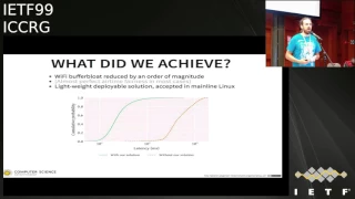
D
Four
point:
nine
through
4.11
and
as
you
can
see,
we
we
saw
this
nice
order
of
magnitude
reduction
in
in
latency
under
load
with
with
the
solution
next
slide.
So
some
of
the
constraints
and
some
of
the
reasons
why
previous
solutions
to
buffer
bloat
do
not
work
well
for
Wi-Fi
bar
these
constraints
in
how
Wi-Fi
works,
and
why
has
the
concept
of
traffic
IDs,
where
packet
going
to
different
stations
have
to
be
Q
together,
so
that
we
can
aggregate
them
at
the
tid
level
and
we
also
need
to
handle
reinjection
of
packets
the
transmission.
D
You
know
we
need
to
run
this
on
really
slow,
really
small
embedded
boxes,
and
we
also
did
not
want
to
modify
the
clients
to
achieve
any
of
this
stuff,
but
especially
the
first
two
points
means
we
cannot
use
the
existing
buffer,
bloat
solutions
for
Wi-Fi,
because
they're
simply
not
capable
of
Duras
next
slide.
So
what
we
did
instead
was
for
the
for
the
queuing
part.
D
We
also
designed
a
scheduler
that
uses
some
of
the
same
techniques
from
if
you
coddle
ADR,
based
scheduler
to
sort
of
make
sure
all
station
should
get
the
same
transmission
time
and
I'm
not
going
to
go
into
the
details
of
how
that
works,
but
you'll
see
it
in
in
some
of
the
year
resort.
Graphs
next
slide
please
so
this
is
this
is
the
Linux
kernel,
peering
structure
and
the
left
here
is
as
before,
and
here
is
after
we
modified
it.
So
the
things
to
notice
here
is
this
curious
layer.
D
This
is
where
you
could
install
your
HMS
beforehand,
but
what
we
have
down
here
at
the
at
the
driver
level
is
another
bunch
of
queues,
and
these
can
be.
This
is
sort
of
the
source
of
the
hundred
milliseconds
of
shearing
latency
that
we
saw
before
so.
What
we
did
was
we
got
rid
of
the
cutest
layer
completely
by
bypassing
it
at
the
at
the
Linux
API
level,
and
then
in
the
in
the
Mac
layer,
which
is
the
the
sort
of
the
library
that
implements
the
Mac
protocol
for
480
to
11.
D
So
this
means
we
now
have
to
manage
to
here
this
way
closer
to
the
hardware.
This
is
only
to
aggregates
which,
depending
on
your
rate,
is
on
the
order
of
10
or
20
milliseconds
enough
cases
next
slide,
then
we
did
some
evaluations
of
this
thing
where
we
sent
data
from
a
server
to
too
fast
clients
on
a
slow
client.
D
This
was
also
to
look
at
the
DSM
fairness
issues
and
we've
we've
used
the
normal
FIFO
queue
which
you
should
all
know
by
now,
this
sucks
and
then
we
have
a
few
kernel
as
sort
of
the
best
we
can
achieve
with
eight
latency,
and
then
we
have
fq
mac
as
the
restructures,
and
then
we
have
the
airtime
vanish
curious
as
the
last
one
and
so
looking
at
the
latency
first
here
we
see
that
we
go
from
of
course
FIFO
this.
This
is
a
large
scale.
D
Obviously,
so
we
go
up
to
almost
a
second
of
latency,
with
with
a
fiber
queue
with
fq
caudal.
We
reduce
it
somewhat
for
the
for
the
fire
stations
we
go
down
to
about
the
50
millisecond
mark
and
then
for
the
fq
mac,
our
nutrient
structure.
We
go
all
the
way
down
to
10
on
20
milliseconds
next
slide.
Please
throughput
also
improves
actually
when,
when
we
apply
this
modifications
and
I'll
go
into
the
reason
for
this
before,
of
course,
just
just
applying
a
few
coddle
actually.
D
So
beforehand,
you
had
a
very
reasonably
small
queue
at
the
very
low
layers,
which
would
tend
to
get
flooded
with
packet,
packets
waiting
to
go
to
the
slow
station,
and
that
meant
that
the
that
the
slow
station
would
take
up
almost
all
of
the
airtime.
In
these
two
cases
it
gets
a
little
better
here
because
you
have
better
curing
or
you
have
round-robin
curing
at
the
upper
layer,
but
just
applying
the
curing
structure
at
the
matte
layer
means
that
we
can
now
have
enough
queue.
D
Space
to
have
always
have
packets
for
for
all
the
stations
available.
So
this
also
this.
This
is
due
to
improved
aggregation
for
the
physicians
and
then,
as
you
can
see,
when
we
apply
the
airtime
scheduler
as
well.
We
get
pretty
much
perfect
airtime
fairness,
even
though
the
the
stations
differ
in
throughput
on
in
raped
by
an
order
of
magnitude.
D
Next
slide,
we
also
evaluated
the
the
impact
on
different
applications
of
these
changes.
We
looked
at
HTTP
load
time
and
we
looked
at
VoIP
performance
by
calculating
synthetic
mass
values
for
the
different
cases,
so
the
HTTP
lost
times,
as
you
can
see
like
this,
is
also
a
large
Delta.
This
is
I
think
35
seconds
to
to
load
a
rather
large
webpage,
which
will
bring
down
to
a
few
seconds
in
the
best
case.
So
this
sort
of
reflects
the
both
the
throughput
and
the
latency.
So
the
small
page
here
is
dominated
by
the
latency.
D
We
can
get
down
to
almost
zero
in
the
best
case,
and
the
large
page
also
gains
more
from
the
from
the
changes
in
throughput,
obviously,
and
next
slide.
So
the
VoIP
test
here,
I'm
not
going
to
go
into
whether
or
not
like
this
actually
corresponds
to
actual
voice
quality.
But
if
we
put
that
aside
from
them
and
assume
that
it
does,
what
you
will
see
here
is
that
FIFO
is
at
1.0
is
completely
unusable
for
best-effort
traffic.
So
this
the
best
effort,
unvoiced
traffic,
is
the
ADA
211
choose
so
in
802
11
you
can.
D
You
have
average
queue
where
you
can
get
priority
at
the
Mac
layer,
and
so
the
thing
to
notice
here
is
that,
with
these
changes
we
now
achieve
better
performance
for
best-effort
traffic
than
we
did
before
with
this
soft
traffic
that
gets
priority
at
the
Mac
layer.
So
this
means
that
we
can
now
run
our
voice
applications
as
best-effort
traffic,
which
is
nice
if
we
do
not
control
the
markings
of
the
package,
so
if
they
are
removed
somewhere
in
transit.
So
this
is
pretty
promising
and
I'm
like.
D
E
Hi
Randall
Jessup
Mozilla,
so
it
looks
like
this
would
have
a
significantly
positive
impact
on
Wi-Fi,
with
WebRTC
in
particular,
because
typically
those
aren't
deserved,
and
so
now
I
would
shoot
the
audio
avoid
law
buffering,
but
also
video
recovery
time
from
packet
losses
or
other
things.
When
you
have
a
round
trip
to
do
it
to
do
an
AK
or
whatever
should
also
be
dramatically
improved,
have
you
done
any
testing
with
WebRTC
yeah
one
other
question
I
had
was
so
there
is
one
downside
to
this,
though
not
may
not
large,
which
is
the
slow
stations.
E
D
Yes,
so
for
the
for
the
first
question:
yes,
we
can
now
run
web
RTC
over
Wi-Fi,
while
other
people
are
using
the
network
and
downloading
and
I
do
this.
Occasionally,
myself,
I,
don't
have
numbers
specifically
for
for
web
apps.
You
see
in
a
test
bed
scenario,
but
but
from
like
I
run
this
code
at
home
and
it
works.
As
for
the
other
thing,
I
think
if
you
go
I
have
some
edge
source
lights.
So
if
you
go
the
other
way
bit
more
bit
more
a
bit
more
at
this
one.
D
About
400
milliseconds
to
almost
2
seconds
of
latency
in
in
the
medium
one
and
a
half
seconds,
so
obviously
we
get
a
lot
of
improvement.
So
if
you
go
back
one
slide,
this
is
this:
shows
you
the
the
difference
in
throughput
when
there's
30
sessions,
so
we
get
sort
of
a
huge
improvement
in
aggregate
throughput.
But
of
course,
if
you
have
a
very
slow
station,
we
are
limiting
it
and
we
do
this
by
basically
starving
it
until
it
slows
down,
and-
and
this
means
this
does
work.
D
But
if
you
are
that
slow
station,
you
are
going
to
notice
I
guess
and
of
course
you
get
it.
You
go
into
sort
of
a
philosophical
argument.
What
notion
of
fairness?
Do
you
really
want
to
to
apply
to
your
network,
and
so
my
reasoning
is
that
since
time
spent
transmitting
on,
Wi-Fi
is
sort
of
the
scarce
resource.
This
is
what
we
should
be
enforcing
fairness
on
where's
the
ADA
to
a
lemon
Mac
by
default
enforces
throughput
fineness,
which
is
why
there's
anomaly
sort
of
appears
in
the
first
place
right.
E
That
I
I
certainly
understand
that
point
of
view
from
a
technical
point
of
view,
from
a
user
level
point
of
view,
that
may
not
be
this
sort
of
fairness
that
they
nest
that
a
user
necessarily
wants
to
apply
depending
on
the
situation.
You
know
there
are
some
intermediate
levels
between
throughput
and
airtime:
fairness,
where
you
allow
slow
stations
to
have
some
level
of
additional
airtime
in
order
to
keep
them
usable.
Okay,
well,
well,
not
overly
hurting
the
fast
stations
and
that
maybe
wasn't.
F
Mccrea
just
to
say
that
the
slow
station
problem
is
also
rather
mitigated.
If
you
have
a
multi
ap
deployment
and
that
dot
11
R
will
tend
to
move
the
slow
stations
to
places
where
they
an
slow,
much
more
vigorously
in
the
presence
of
air
time
fairness.
And
so
actually
you
get
better
throughput
as
seen
from
the
station.
If
there
is
an
alternate
ap,
it
can
talk
too.
C
G
Thanks
Jenna,
so
my
name
is
Neil
Caldwell
and
I'm
gonna
give
a
quick
update
on
the
VBR
congestion
control
project,
and
this
is
joint
work
with
my
colleagues
at
Google,
including
you
Chun
and
Stephen
Sohail,
the
quick
PPR
team,
which
is
in
and
our
illustrious
co-chair,
chana
and
Victor,
and
then
Ben
Jacobsen
as
well.
Next
slide,
please!
So
just
a
quick
outline
of
what
I
wanted
to
cover
we're
gonna
start
with
a
quick
review
of
bbr
and
its
background.
If
you
want
more
details,
there
are
some
links
to
previous
IETF
presentations.
G
G
I'm
gonna
speak
briefly
about
active
and
upcoming
work
for
bbr,
because
we,
you
know
there
are
still
things
that
we'd
like
to
improve
about
it
and
then
I'm
going
to
give
a
quick
deployment
update,
which
the
the
news,
here
being
that
we've
switched
a
quick
traffic
from
Google
and
YouTube
over
to
using
VBR.
Just
next
slide,
please
so
just
a
quick
background.
G
The
the
motivation
for
the
bbr
project
is
really
the
issue
sort
of
fundamental
issues
we
see
with
loss
based
congestion,
control,
meaning
Reno
and
cubic
largely,
and
basically
the
issue
is
that
packet
loss
is
not
really
a
good
proxy
for
congestion.
These
algorithms
sort
of
assume
that
packet
loss
is
equivalent
to
congestion.
But
of
course
that's
that's
not
the
case
and
really
bites
us
in
a
couple
of
important
use
cases.
G
There
are
some
examples
here
so,
for
example,
to
get
10
gigabits
over
a
100
millisecond
round-trip
time.
You
need
less
than
1
packet
loss
per
30
million
packets,
which
is
tough
to
achieve
operationally,
and
if
we
look
at
more
realistic
loss
rates
that
we
see
over
the
internet
or
over
high-speed
winds
with
commodities
switches
as
shallow
buffers,
then
you
see
more
like
a
1
percent
loss
rate
and
there,
with
100
millisecond
round-trip
time
you're
going
to
get
around
3
megabits,
with
the
loss
based
congestion
control
at
the
other
end
of
the
spectrum.
G
G
It
does
also
have
a
see,
end
back
stop,
but
it
tries
to
do
most
of
its
action
with
pacing,
whereas
the
other
previous
congestion
controls
are
built
around
a
seal
in
this
sort
of
limits.
The
volume
of
data
in
flight
next
slide,
please
alright,
so
I
want
to
dive
into
the
first
internet
draft
that
we
posted
a
couple
weeks
ago.
This
is
the
delivery
rate,
estimation
internet
draft
and
there's
a
link
there
or
you
can
google
it
if
the
slides
are
not
up
yet
so.
G
Basically,
the
the
idea
here
is
that
on
every
ACK,
the
this
algorithm
provides
a
sample
that
has
two
aspects.
The
first
is
an
estimated
rate
at
which
the
network
delivered
this
most
recent
flight
of
data
packets.
Then
the
second
aspect
is
it
tells
you
whether
or
not
that
particular
rate
sample
was
application
limited
by
the
sender.
That
is
the
sending
app
ran
out
of
data
to
send
at
some
point
during
that
flight,
and
why
did
we
separate
this
out
into
a
separate
draft?
G
G
Also,
you
can
implement
the
bandwidth
sampling
separately
and,
in
fact,
in
the
Linux
TCP
code,
it's
definitely
a
separate
algorithm
and
then
finally,
it's
also
useful
to
think
about
bandwidth
estimation
outside
of
the
context
of
congestion,
control
or
outside
of
the
context
of
VBR,
the
other
congestion
control
algorithms,
where
I
want
this
or
adaptive
bitrate
streaming.
I
want
this,
for
example,
to
pick
which
bitrate
to
show
the
user
next
slide,
please.
So
the
the
basic
design
principles
that
we
were
working
from
for
this
bandwidth
estimator
were
first.
G
We
wanted
it
to
be
purely
passive
in
the
sense
that
we
wanted
it
to
work
with
the
acknowledgments
that
were
already
going
to
receive
for
the
the
data
that's
in
flight
for
that
transport
connection.
Second,
we
wanted
it
to
be
generic.
It's
in
portable
two
different
congestion
control,
algorithms,
different
transport
protocols,
and
so
far
we
have
a
Linux
TCP
implementation,
a
quick
camp
implementation
and
then
there's
a
FreeBSD,
a
TCP
implementation
underway
at
Netflix
as
well,
and
we
wanted
to
also,
as
I
said,
track
which
samples
were
application
limited.
G
We
wanted
it
to
be
relatively
efficient,
so
constant
time
for
each
act
that
comes
in.
We
wanted
to
try
to
err
on
the
side
of
being
conservative
and
underestimate.
We
wanted
to
make
sure
that
we
got
feedback,
whether
we're
in
recovery
and
getting
sax
or
we're
not
and
we're
getting
cumulative
acts
are
to
make
sure
we
can
try
to
get
an
estimate
at
all
times,
and
then
we
wanted
to
try
to
get
an
estimate
that
is
over
a
time
scale.
G
That
is
at
least
runaround
trip,
rather
than
one
packet
to
try
to
filter
out
some
noise
and
if
we
think
about
alternatives,
the
main
alternatives
out
there.
For
bandwidth
estimation,
we
considered
were
we're
sort
of
packet,
dispersion,
metrics,
looking
at
the
interacts
facing,
and
there
are
various
approaches
in
that
space,
packet
pair
packet,
trains
and
chirping.
But
some
of
the
challenges
we
saw
with
those
kinds
of
approaches
are
that
you
know
in
the
real
world,
with
cable,
modems
and
Wi-Fi
and
cellular
links.
There
are
a
lot
of
things.
G
So
if
we
take
down
to
the
very
essence
of
the
delivery
rate,
estimator
I
think
this
is
a
good
picture
to
keep
in
mind
the
The
Cove
here
that
we're
drawing
has
on
the
y-axis
the
amount
of
data
that
it's
been
cumulatively
cumulative
Leaney
delivered
over
or
acknowledged
as
delivered
over
the
lifetime,
the
connection
and
then
on.
The
x-axis.
G
We've
got
time,
that's
elapsed,
and
what
we're
really
trying
to
show
here
is
the
essentially
the
slope
of
the
delivery
curve,
and
a
key
part
here
is:
what
is
the
time
interval
over
which
we
are
calculating
that
slope
and
the
key
issue
here
is
that
we
we
calculate
the
the
time
interval.
We
calculate
this
slope
over
time
interval
that
starts
from
the
most
recent
act
that
we
have
received
before
we
sent
a
packet
until
the
ACK
for
that
packet.
B
G
B
G
We
go
back
to
the
previous
slide,
so
the
the
data
I
didn't
do
the
data
packet
in
question
here
that's
being
sent.
Is
this
one
here
and
that's
act
here,
and
then
we
go
back
to
the
act
that
was
sent
before
Paquette
and
we
use
that
as
the
start
of
the
this
great
sample,
and
then
we
just
basically
calculate
an
accurate.
G
That
is
the
amount
of
data
that
was
delivered
between
those
two
acts
divided
by
the
time
elapsed
between
those
two
acts
to
give
us
that
slope
and
that's
the
act
right
from
this
algorithm
next
slide.
So
you
might
want
you
might
ask
well
why
can't
we
just
use
the
rtt
and
what
happens
is
if
you
try
to
calculate
an
accurate.
That's
just
the
amount
of
data
delivered
divided
by
the
RTT.
G
You
can
see
if
we
look
at
the
same
picture
with
that
alternative
attempt
at
calculating
in
a
crate
that
actually
gives
you
an
accurate
that
sort
of
badly
overestimates
the
the
actual
delivery
rate,
because
it
doesn't
incorporate
the
amount
of
time
that
was
really
needed
by
by
the
network
to
deliver
all
those
bytes
that
you
are
accounting
in
your
sample
there
all
right
next
slide.
So
one
big
issue
that
you
run
into
when
trying
to
calculate
delivery
rates
in
the
real
world
is
what
you
might
call
act
compression.
G
There
are
similar
effects
going
by
other
names
that
are
have
similar
issues.
Aggregation
decimation
stretch
acts
basically
by
all
of
these,
with
all
of
these
kinds
of
effects.
We
have
acts
that
are
delayed,
and
then
they
arrive
in
a
burst
or
there's
a
single
act
that
covers
a
lot
of
data
that
was
delivered
and
this
can
be
caused
by
the
receiver
can
be
caused
by
the
middle
box.
But
the
big
issue
is
that
these
are
quite
frequent
in
the
real
world.
G
They're
really
common
in
Wi-Fi,
cellular,
cable,
modem
links
and
the
issue
is
that
you
can.
If
you're,
not
careful,
you
can
run
into
excessive
I,
create
samples,
so
I'll
give
an
example
here
on
the
next
slide.
So
here's
a
real-world
trace
where
the
actual
bandwidth
was
something
like
8.9
megabits,
but
the
a
crate
sample
shown
in
red
here
is
27
megabits,
and
that's
because
of
the
act
compression
that
you
can
see.
There's
a
horizontal
green
section
in
the
cumulative,
the
ACK
stream.
G
So
the
way
that
the
algorithm
currently
deals
with
this
is
to
sort
of
simply
filter
out
the
accurate
samples
that
are
impossibly
high
using
the
following
observation.
So
basically,
the
accurate
can't
really
physically
exceed
the
send
rate
on
a
sustained
basis
for
obvious
reasons,
and
so
what
you
can
do
is
for
each
flight
of
data,
that's
delivered
between
sun
sand
and
some
ACK.
You
can
calculate
the
send
rate
for
that
flight,
and
then
you
can
calculate
accurate
for
that
flight
and
then
to
help
filter
out
these
implausible
samples.
G
You
can
just
use
as
the
delivery
rate
simple
the
minimum
of
the
send
rate
and
the
a
crate,
and
this
tends
to
do
a
good
and
good
enough
job.
In
most
cases,
it
can
be
improved.
It's
not
perfect.
It
can
be
improved
to
filter
out
more
thoroughly.
Some
of
these
implausible
a
crates
and
it's
an
active
area
of
work
for
the
team.
G
Next
slide,
John
if
you
get
a
sec.
Thank
you.
So
what
this
looks
like
on
the
picture
is
if
we
take
that
same
example,
here
we
would
look
at
the
a
crate
which
were
I
previously,
showed
you
and
then
the
the
son
rate,
which
is
shown
here
in
red,
and
in
this
case
we
would
use
the
min
of
the
two,
which
is
is
the
son
rate,
and
that
gives
us
a
safe,
in
this
case
that's
sort
of
an
under
estimate,
but
at
least
we
haven't
overestimated
and
probably
the
congestion
control
algorithm.
G
Certainly
if
it's
bbr
we'll
be
able
to
filter
this
out
appropriately,
all
right
so
I'm
going
to
quickly
zoom
through
some
pictures
and
go
into
the
detailed
notation
here.
This
is
mostly,
if
you're
reading
the
internet
draft
at
some
point,
and
you
want
to
know
what
picture
can
explain
a
particular
equation
that
you're
looking
at
you
can
go
back
to
these
slides.
So
this
is
just
a
quick
way
to
show
what
the
sundry
it
looks
like
it's.
G
Basically,
the
slope
of
this
Green
Line,
it's
the
amount
of
data,
that's
acknowledged
as
delivered
divided
by
the
send
elapsed
time
the
amount
of
time
it
took
you
to
sent
that
send
that
data
next
slide.
Correspondingly,
the
accurate
is
just
the
amount
of
data
acknowledged
it's
delivered
divided
by
the
time
it
took
to
a
call
those
packets
next
slide.
G
The
delivery
rate
is
just
the
minimum
of
those
two
rates
next
slide.
So
the
other
thing
I
said
that
this
estimator
provides
is
a
notion
of
whether
a
rate
sample
was
application
limited
or
not,
and
it's
a
it
does
this
with
the
algorithm
a
you
could
sort
read
in
detail
in
the
in
the
draft
which
all
zoom
by
here,
but
basically
it.
Let
me
go
up
to
the
next
slide
and
this
chart
shows
you
a
picture.
G
Basically,
every
time
the
application
runs
out
of
data
to
send
in
marks
the
application
as
a
limited
and
then
when
all
of
those
acclimated
samples
have
are
out
of
the
pipeline,
then
we
can
exit
that
preparation
where
the
samples
are
marked
application
limited.
And
then
we
can
get
back
into
this
blue
region
where
we've
got
non
application,
limited
samples,
basically
in
the
interest
of
time,
I'll
skip
over
the
details.
G
But
the
idea
is
that
when
your
application
limited,
you
go
to
sort
of
idle
or
silent
bubble
in
the
pipeline,
and
you
just
need
to
track
when
that
pipe
when
that
bubble
has
been
acknowledged
and
it's
no
longer
in
the
pipe
no
longer
pulling
down
on
your
your
rate.
Samples
next
slide.
So
let's
go
move
on
the
bbr,
so
the
big
picture
here
for
bbr
is
that
it
takes
as
input
these
bandwidth
or
rate
samples.
G
And
then
those
two
estimates
get
fed
into
a
sort
of
probing
state
machine
that
increases
and
decreases
in
flight
to
try
to
keep
a
reasonable
number
of
packets
in
the
pipe
and
also
also
feed
samples
back
into
that
model
and
the
output
of
that
state
machine
and
all
that
together
is
a
pacing
rate
and
a
pacing
quantum.
A
chunk
size
that
you
want
to
use
for
your
pacing
and
a
congestion
window.
G
Our
maximum
amount
of
data
you
want
to
have
in
flight,
then
that
goes
into
the
pacing
engine,
which
chops
up
the
data
stream
into
those
quantum
into
those
quanta
and
then
paces
them
out
at
the
given
rate
and
makes
sure
that
the
volume
of
data
never
exceeds
that
congestion
window
next
slide.
And
so
here's
a
quick
outline
of
what
we
cover
in
the
internet
draft.
It's
basically
a
lot
of
the
same
stuff
I.
Just
showed
in
the
picture
so
I'll
try
to
breeze
right
through
it.
G
We
cover
the
network
path
model,
both
bandwidth
and
round-trip,
propagation
time.
We
cover
the
target
operating
point,
which
is
that
we
want
to
try
to
maintain
both
rate
balance
to
try
to
match
the
available
bottleneck
bandwidth
using
our
pacing
rate,
and
then
we
also
try
to
achieve
a
full
pipe
to
try
to
keep
the
amount
of
in-flight
data
roughly
equal
to
the
estimated
bandwidth
delay
product
for
our
flow.
And
then
we
use
the
control
parameters
at
our
disposal.
G
G
So
there's
the
warmup
period
when
we're
we've
got
a
fresh
new
connection
and
we've
got
this
issue
that
bandwidth
sort
of
spans.
You
know
10
or
11
orders
of
magnitude
from
bits
per
second
up
to
hundreds
of
gigabits,
so
we
want
a
rapidly
probe
of
the
network.
We
do
that
in
the
startup
state,
where
we
exponentially
ramp
up
our
sending
rate,
doubling
it
each
round-trip
time
as
long
as
the
delivery
rate
is
also
doubling,
and
then
we
look
for
a
full
pipe
using
a
sort
of
looking
for
a
plateau
in
the
delivery
rate.
G
And
then
when
we
asked
omit
that
we
fill
the
pipe,
we
enter
the
state
called
drain
where
we
cut
the
pacing
rate
to
below
the
estimated
bandwidth
so
that
the
in-fight
amount
of
the
in-flight
data
is
sort
of
gradually
or
other
quickly
really
trains
out
of
the
network.
Until
we've
estimated
that
we've
pulled
our
in-flight
data
down
to
the
bandwidth
filet
product
and
at
that
point
we
sort
of
go
into
steady-state,
where
we
do
the
same
kind
of
probing,
but
on
a
more
gentle
amplitude.
G
So
the
probe
bandwidth
state
cycles,
the
pacing
rate
up
and
down
to
do
that
probing
for
bandwidth
and
then
draining
the
queue
and
then,
if
needed,
then
we
can
also
do
sort
of
coordinated
cut
in
in-flight
to
probe
for
the
round-trip
propagation
delay.
And
then
the
details
for
all
of
those
mechanisms
are
in
the
in
the
draft.
Next
slide,
please
so
we're
not
done
with
VB.
Are
we?
We've
got
a
lot
several
things
that
we'd
like
to
improve
several
known
issues
or
known
scenarios
where
we
definitely
want
to
get
the
behavior
to
be.
G
We
want
to
improve
the
behavior,
so
the
the
biggest
focus
right
now
or
one
of
the
big
focuses
right
now
is
on
soon
areas
where
there
are
high
degrees
of
AK
aggregation,
and
we
want
to
improve
both
the
bandwidth
estimate-
and
you
know,
as
we
mentioned
earlier,
you
can
get
bandwidth.
Those
were
estimates
in
these
cases
and
we're
working
on
new
techniques
for
filtering
out
these
variations
and
getting
a
more
reliable
bandwidth
estimate
in
these
cases
and
then
the
second.
G
We
want
to
make
sure
that
we're
provisioning
enough
data
in
flight
in
these
cases
is
when
you
get
these
ACK
a
grinning
cases.
You've
got
often
you
got
a
very
long
silence,
sometimes
tens
of
milliseconds,
even
if
you're
a
minimum
round-trip
time
is
one
millisecond.
You
might
wait.
10
20
40
milliseconds
for
an
ACK,
and
so
you
have
to
make
sort
of
just
estimation
of
how
much
data
you
want
to
have
in
flight.
G
Given
that
behavior
and
then
another
area
of
work
is
BB
behavior
and
shallow
buffers,
there
are
some
known
issues
where
VBR
can
keep
considerably
more
data
in
flight
that
you'd
like.
If
there
are
shallow
buffers,
it's
still
bounded
to
an
estimated
PPP.
But
if
there's,
if
you
don't
have
a
BD
P
of
Q
to
hold
that,
then
the
packet
rate
packet
loss
rate
can
be
higher
than
we'd
like
to
see.
G
So
that's
a
known
issue
or
there's
active
work
and
discussion
and
testing
on
the
PBR
dev
list
and
then
finally,
there's
also
work
underway
if
to
look
at
B,
be
ours
behavior
in
data
center
environments,
where
there
are
large
numbers
of
flows
next
slide.
So
in
conclusion,
there
are
two
new
bbr
drops
out:
we're
happy
to
get
people's
feedback
suggestions,
questions
whatever
we'd
love
to
hope
to
see
he
back.
The
PBR
is
now
deployed
for
quick,
as
I
mentioned,
on
google.com
in
YouTube.
G
That's
the
latest
deployment
update
and
the
character
of
the
results
is
similar
to
those
results
we
saw
for
TCP,
which
we
mentioned
the
last
IETF.
So
with
that
now
we
have
basically
all
Google
and
YouTube
servers.
Talking
to
the
outside
world
and
then
the
Google
Data
Center,
when
traffic
and
our
backbones
between
our
data
centers
that
way
in
traffic
is
also
using
PBR,
and
then
we
see
better
performance
than
Kubik
for
web
traffic,
video
traffic
and
RPC
traffic.
G
The
code
is
available
as
open
source
with
links
in
the
slides
and
then
work
is
underway,
as
I
said,
for
FreeBSD
as
well.
You
can
talk
to
the
Netflix
folks
and
then
we're
actively
working
on
improving
the
VBR
algorithm,
as
I
mentioned,
and
we're
always
happy
to
hear
test
results
or
look
at
packet,
races
and
next
slide,
and
that's
it
if
we
basically
have
a
landing
page
here
on
the
mailing
list.
So
if
you
search
for
PBR
dev
you'll
get
the
mailing
list,
which
has
intro
message
that
has
links
to
the
internet
drafts
the
paper.
E
To
two
quick
questions:
the
small,
the
small
buffer
issue
that
still
you're
so
looking
at,
does
that
also
include
looking
at
things
like
aqm,
various
variations
on
aqm
and
how
well
that
work
and
what
the
second
thing
is.
Have
you
done
any
comparisons
with
the
some
of
the
proposed
algorithms
for
armed
cat
or
how
well
it
coexists
with
the
armed
cat,
algorithm
or
planning
to
do
that.
G
Yeah,
so
the
the
work
looking
at
shallow
buffers
would
also
in
that
effort
also
includes
a
QM
I
guess
so
far.
We've
done
tests
with
with
PI
and
Caudill.
If
other
people
have
other
algorithms
out
there
they'd
like
to
see
testing
with,
let
us
know
or
you,
obviously
you
can
do
the
tests
as
well
so
yeah.
We
are
definitely
looking
at
a
QM
as
well
as
Java
buffers,
since
they
have
so
much
in
common.
Obviously,
and
then
we
have
not
yet
done
tests
with
coexistence
with
RM
cat.
That's
definitely
something
that
we
like
to
do.
H
E
C
Anger,
this
is
a
deeper
conversation,
I
think
not
not,
because
so
I
think
Reno
for
for
quick
makes
sense
at
the
moment,
because
the
simplest
thing
to
talk
yes-
and
it
gives
you
completeness,
but
I
do
think
that
there's
something
to
be
said
about
actually
and
I've
talked
about
this
in
the
past-
about
not
actually
having
standards
track.
Condition
controllers
at
all
and
having
transports
rely
on
sort
of
condition,
controllers
that
are
documented
elsewhere.
So.
H
I
C
G
I
And
we
used
that
one
for
our
student
reading
group
at
Akamai
and
I
kind
of
quite
enjoy
talking
about
it.
Okay,
but
I
was
struck
by
I,
didn't
see
a
lot
of
evaluation
or
commentary
from
your
you
as
authors
on
prior
work.
Do
you
know,
for
instance,
the
one
that
I
brought
up
the
students
was
the
2007
work
by
Cola
and
in
Mary
Vernon
called
TCP
Madison
that
as
a
model
based
one
yeah
I
thought
it
was
a
nice
comparison.
I
Thank
you.
I'll
certainly
do
that
one,
and
it
was
also
a
UDP
based
implementation
application.
The
one
thing
I
can
offer
that
you
did
definitely
improve
upon
is
there's
require
to
change
in
the
receiver.
They
they
they
could
force
an
ACK
yeah,
and
that
was
the
other
aspect
about
where,
where
are
you
guys
in
deciding
that
you're
just
doing
something?
That's
based
on
empirical
things
about
what
the
real
Internet
today
is
doing
versus.
What
would
you
ideally
like
to
change
in
the
receiver
that
could
make
this
maybe
better
right.
G
Yeah,
no,
that's
a
good!
That's
a
good
question
yeah,
so
we
wanted
to
start
with
something
that
could
work
with
the
deployed
receivers
that
are
out
there
now,
because
we
we
did
want
something
that
would
work
for
both
TCP
and
quick,
but
that's
very
good
point
that
there's
probably
a
lot
of
leverage
to
be
gained
if
you're,
if
you
have
a
receiver
population
that
you
can
iterate
with
quickly,
so
there
are
plans
to
look
at
what
we
can
gain
by
a
receiver
side.
G
J
Shaky
Versova,
Dean
I
was
curious
about
what
Sabine
del
develop
meant
on
when
you
don't
have
enough
packet
in
flies
to
make
up
a
reliable
estimation.
For
example,
if
you
have
a
sort
of
Bart
is
traffic
like
videos
like
where
you
transmit
a
bars,
and
then
you
wait
and
then
get
another,
and
maybe
between
one,
the
other.
You
don't
have
enough
data
to
estimate
the
round-trip
or
the
throughput.
What's
the
state
of
the
organ
at
this
point,
what
is
traffic
department?
J
G
The
algorithm
as
it's
currently
structured
does
not
do
anything
special
in
those
cases.
What
it
would
end
up
doing
is.
It
would
start
out
with
the
initial
congestion
window
picked
by
the
transport
implementation.
Usually,
you
know
initial
push
condition
when
you
have
ten
packets
and
then
it
would
from
there
it
would
calculate
an
initial
pacing
rate
using
the
regular
using
the
hi.
What
we
call
the
high
gain
that
can
double
the
rate
every
round-trip
time,
which
is
two
point,
eight
nine.
So
it
would
calculate
two
point:
eight
nine
times
the
initial
window
per
round-trip
time.
G
So
those
low
application,
limited
rate
samples
shouldn't
cause
it
to
decrease
its
sending
rate.
So
it
should
should
be
on
the
whole
for
application.
Limited
traffic
like
that,
it
should
be
on
the
whole,
pretty
similar
to
what
you
would
get
with
Reno
or
cubic
in
terms
of
the
overall
bit
rate.
I
would
think
all
right.
C
K
Thanks
for
inserting
me
into
the
agenda
talk,
so
my
name
is
Ron
Bess
and
I'm,
presenting
some
measurements
that
we
did
just
only
a
brief
heads-up.
This
is
joint
work
with
Mario
Martina,
so
we
did
some
experiential
evaluation
in
the
small
testbed,
using
our
speeds
of
one
gigabit
and
ten
gigabit
per
second
based
on
the
Linux.
Our
4.9
version
of
EBR
and
the
testbed
looks
like
this,
where
we
have
sender
with.
K
Basically,
if
we
10
gigabit
interfaces
software
based
switch
in
the
middle
and
the
receiver,
which
is
connected
by
one
gigabit,
even
as
interface,
the
round-trip
time
was
20
milliseconds
and
we
use
the
small
buffer,
which
is
corresponding
to
0.8
VD
P
Mo's.
So
the
this
is
only
brief.
Heads
up
heads
up
on
presentation,
so
the
full
results
will
be
in
a
research
paper
at
the
ICMP
17
and
first
we
tried
to
show
that
VB
is
working
correctly
in
this
setup,
so
single
flow
works
as
expected.
So.
E
K
We
get
the
the
whole
throughput
here
of
the
bun
elect
link
and
also
you
can
see
the
the
RTT
is
kept
somewhere
around
the
base
RTT.
So
we
have
the
the
probing
phases
here,
the
gain
cycling
and
then
here
for
examine
the
probe
RCT.
So
yeah,
that's
working
well,
but
situation
changes
if
we
use
multiple
flows
here.
In
this
case,
we
used
six
PBR
flows
to
per
interface
and,
as
you
can
see,
this
year
is
Sanders
transmission
rate.
K
Actually
in
the
purple
line
here
is
the
total
amount
or
the
aggregate,
and
that's
way
above
one
gigabit
per
second,
so
VR
is
more
or
less
in
this
case,
a
little
bit
too
aggressive
and
since
is
just
neglects
packet
loss
as
congestion
signal.
It
doesn't
back
off
here
so
in
comparison
to
that
next
slide.
K
Please
cubic
works
as
expected
here,
so
it
doesn't
send
faster
than
useful,
and
here,
in
this
case
on,
you,
can
also
see
it
by
the
numbers
like
cubic
retransmissions
for
small
buffers,
also
here
for
10
gig
per
second,
for
example,
in
comparison
to
bbr.
That's
some
orders
of
magnitude,
so
you
know
from
our
perspective,
maybe
I
neglecting
packet
loss,
as
congestion
is
maybe
not
not
the
way
to
go.
K
L
This
is
a
long
pragma
from
paper.
I've
also
been
experimenting
with
BB,
r
and
I've,
seen
that
in
some
percent
of
the
cases
with
even
two
or
three
flows,
it
gets
into
this
type.
Well,
one
flow
will
get
very
high
throughput
and
the
other
flow
we
get
like
110
to
130
put
another
case.
If
we're
one
from
ABR,
we
think
on
you
know,
there's
losses,
but
I
would
say
it's
not
congested
and
the
other
of
flows
will
you
know
completely
back
half
from
that.
So
I
also
have
some
concerns.
I.
G
Yeah
I
want
to
thank
you
all
for
this
work
and
I.
Just
want
also
want
to
note
that
these
are
the
issues
that
have
been
mentioned
are
well
known
and
have
been
discussed
on
the
VBR
dev
mailing
list.
I
would
encourage
people
to
subscribe
to
the
mailing
list
and
and
check
out
the
discussions
there.
People
the
you
there.
Definitely
this.
This
issue
that
you
raise
here
is
the
the
one
I
was
referring
to
earlier
in
my
presentation
about
PBRs,
behavior
and
shallow
buffers,
and
this
is
definitely
an
active
area
of
research
focus
for
our
group.
C
C
M
M
So
in
the
sender
only
there
is
a
clear
migration
towards
bbr,
which
is
mostly
delay
based
I
could
say,
and
there
is
also
the
concern
about
ignoring
drop.
But
of
course
there
is
a
network
today,
which
is
usually
not
supporting
a
lot.
There
is
no
easy
end.
There
is
hardly
any
aqm,
so
it's
the
obvious
thing
to
do.
On
the
other
hand,
there
our
actions
going
on
in
the
aqm
working
group,
the
second
layer
where
we
have
pi
by
square
f
q,
Caudill,
okay,
next
slide
so
also
quite
obvious.
M
We
all
want
to
improve
throughput
and
avoid
buffered
blood,
and
in
the
third
case
we
also
want
to
have
really
low,
latency
and
a
new
class
and
to
be
compatible
with
Torino.
That
was
the
original
strategy.
So
next
slide.
If
we
look
more
detailed-
and
we
also
did
some
experiments-
this
is
how
bbr
works
on
tail
drop.
M
We
did
a
test
compared
on
hundred
megabit
link
on
20
milliseconds
round-trip
time,
so
an
bbr.
It's
actually
it's
quite
good
work
and
it
works
very
well.
It
can
achieve
high
throughput
and
full
link
utilization.
So
this
is
so.
We
have
here
four
flows,
long
running
flows
and
they
evenly
use
the
link
capacity,
and
here
we
have
about
hundred
requests
per
second.
M
Exponential
distribution
above
arrival
time
and
a
Pareto
distribution
of
size-
and
this
is
the
completion
time
so,
and
the
minimum
based
on
the
round-trip
time
is
quite
low
and
and
also
the
maximum
is
limited.
So
that's
that's.
Okay
and
the
queue
size
is
also
around
20
milliseconds
minimum,
because
bbr
is
more
like
trying
to
measure
what
is
the
minimum
packets
in
flight
and,
what's
and
forces
a
little
bit
its
amount
of
packets
and
everything
which
is
above
that
is
stacked.
M
M
Quite
at
the
target
here
is
15
milliseconds
on
a
PI,
a
cone,
and
there
is
with
a
reasonable
drop
probability
of
0.01%
drop.
We
can
keep
the
queue
at
15
milliseconds
and
the
dynamic
flows.
They
have
also
a
good
completion
time.
There
are
some
limited
loss
and
you
see
that
the
the
dynamic
flows
are
actually
moderated
around
the
15
Mille
second
target,
so
that
you
could
say
it's
a
bit
better
or
worse.
It
depends
on
your
perspective,
of
course,
next
slide.
This
is
where
we
have
data
center
TCP
on
a
step,
a
queuing.
M
So
it's
also.
How
do
you
could
work
in
in
alpha
rest
mode?
There
you
see
that
the
completion
time
is
really
low.
Latency.
The
queue
is
with
stepped
result
of
one
millisecond
very
low.
The
the
other
thing
is
that
the
variations
in
for
dynamic
traffic
or
modulated
below
the
queue
size
so
and
it's
hitting
a
little
bit
on
the
on
the
utilization.
So
that's
another
compromise,
but
it's
guarantees
you
really
low
latency
no
drop
at
all.
M
So
that's
the
other
part,
so
all
of
them
have
their
advantages
and
their
possibilities
next
right,
but
there
are
some
concerns,
and
so
initially
there
was
with
reno
2
cubic
some
compatibility
with
with
drop,
but
today
indeed
like
like
was
mentioned,
there
is
no
compatibility
with
drop
and
there
is,
of
course,
then
a
kind
of
detachment
between
what's
going
on
in
this
layer
where
we
have
a
clamps
and
in
this
layer
where
we
also
want
to
be
compatible
with
reno.
So
in
the
next
slide.
M
Here
is
an
example:
what
happens
if
you
put
bbr
on
top
of
an
ATM,
so
bbr
sets
the
target
to
20
milliseconds
and
the
aqm
sets
the
target
to
15
milliseconds.
So
it's
the
same
as
before,
and
of
course,
bbr
sets
its
target
and
the
pi
will
increase
the
probability
until
finally,
usually
VBR
detects
the
bottleneck
as
a
pacer
at
the
moment,
and
there
are
very
high
drop
probabilities,
and
even
so
you
see
here
the
drop
probability.
M
It
is
around
5
to
10%
for
several
tens
of
seconds
and
then
only
1%
for
the
other
tens
of
seconds.
So
this
is
a
problem,
that's
right.
So
if
we
don't
do
anything,
it
will
force
actually
operators
to
disable
a
queuing
at
the
moment,
and
we
did
also
a
tzn
because
it
needs
an
AKM.
So
it's
a
bit
of
a
problem
and
a
concern.
We
think
and
it
should
have
a
solution
and
in
the
next
slides,
a
possible
solution
could
be
because
it's
actually
not
a
problem.
M
Well,
actually,
both
we
want
to
solve
the
same
problem.
Bbl
wants
to
have
as
one
of
these
main
objectives
high
throughput
under
higher
and
trip
times
and
high
loss
conditions,
but
also
offer
s.
We
want
to
be
compatible
with
the
classic
TCP,
but
we
don't
want
to
be
compatible
with
the
pathological
cases.
So
we
also
want
to
have
high
throughput
under
these
circumstances.
M
So
as
a
possible
solution,
we
were
thinking
on
already
four
l4s,
but
it's
equally
applied
applicable
for
four
PBR
to
have
round
trip
time,
independence
above
a
certain
round
trip
time,
so
that
a
flow
with
hundred
milliseconds
could
be
as
aggressive
as
a
flow
of
five
milliseconds.
Today,
bbr
is
already
having
an
opposition
or
an
opposite
dependency
on
the
round
trip
time.
So
it's
more
aggressive.
The
bigger
the
round
trip
time
so
to
be
equally
aggressive,
is
at
least
a
good
compromise.
M
On
the
other
hand,
we
also
want
to
be
less
responsive
for
hydrops,
so
at
a
certain
probability,
bottleneck
or
below
a
certain
probability
of
the
network.
Why
not
be
scalable
at
that
point
so,
for
instance,
if
we
make
make
classic
congestion
control
responsive
in
a
scalable
way
below
1%,
we
could
always
get
around
24
drops
per
second
a
very
frequent
signal,
also
with
the
round
trip
time
dependence.
If
you
have
1%
drop,
you
could
also
get
30
megabits
per
second,
which
is
a
Hydra
probability
1%,
and
you
get
reasonable
high
throughput
as
well.
M
So
if
next
slide
here,
for
instance,
if
we
have
round
trip
time
independence
above
5
milliseconds
in
this
case,
you
will
see
this
is
throughput.
So
this
is
usually
a
rate,
and
there
are
two
types
of
rates:
there
is
the
rate
of
the
traffic
itself
and
is
the
rate
of
the
marks,
so
how
many
marks
per
second
you
get
so
there's
these
set
of
lines
operate.
M
These
sets
of
lines
are
the
the
the
drops
per
second,
you
could
say
and,
as
you
can
see,
what
we
proposed
is
to
limit
it,
so
to
always
have
24
drops.
Second,
if
800
milliseconds
and
1%
drop
probability
in
general,
the
Reno
and
the
cubic
so
we're
having
here
Reno
in
cubic
lines,
the
bottom
lines
here
they
have
around
one
drop
per
minute,
which
is
not
that
much
and
it's
even
going
worse.
M
With
that
amount
of
drop
probability,
there
will
always
be
at
least
30
megabits
per
second
of
throughput.
That
could
be
achieved.
Of
course
we
can
discuss
about
what
should
be
the
real
thresholds
or
real
values
of
these
settings,
but
okay
in
the
next
slide,
the
resource
shown
previously,
you
saw
here
the
round-trip
time.
Here
is
the
probability
so
here's
this
hydro
probability
and
although
rate
and
here
is
a
low
drop
probability
with
where
we
expect
to
have
high
rates.
So
if
we
see
that
Reno,
this
is
the
bottom
line
here,
the
throughput
is
limited.
M
M
N
M
We
could
go
up
to
200
kilobits
per
second,
so
on
the
1%
case
here
you
again
have
the
24
drops
per
seconds
and
a
30
megabit.
So
if
you
become
scalable
here,
you
can
have
much
higher
throughputs,
where
okay,
the
throughput
can
be
very
high,
but
this
amount
of
drop
probability
means
that
you
only
get
two
drops
per
hour
or
after
or
one
drop
every
two
hours.
M
So
we
we
have
a
paper,
it's
not
a
published
paper.
It's
it's!
It's
on
a
website
describing
all
the
different
scalability
requirements
and
I've
talked
about
those
two.
They
were
initially
meant
to
be
in
the
context
of
Alvarez
but
of
course,
they're
also
applicable
in
in
the
classic
DCPS.
So
if
you
want,
you
can
read
more
in
this
paper,
we
can
also
have
discussions
about
this.
If
you
are
interested
in
more
of
these
experiments,
there
are
a
few
big
videos
that
I've
pushed
to
youtube.
Where
you
can
see
also
experiments.
O
O
We've
got
a
lot
of
code
that
tries
to
solve
all
these
problems
and
we
feel
we're
still
on
the
right
direction,
but
I
wanted
to
try
and
just
explain
the
problems
and
because
they're
they're
actually
problems
that
haven't
really
been
articulated
here
before
so
the
first
one.
If
you
look
at
the
utilization
of
three
GE
vs.
O
O
But
that
was
because
of
a
combination
of
the
problem
here,
that
of
the
variation
of
the
capacity
versus
the
congestion
control
and
a
problem
with
the
receive
window
attuning
where
the
auto-tuning
couldn't
cope
with
the
dynamics
either
so
you're,
actually
getting
only
43
percent
utilization
of
a
4G
network
and
that
that
was
measured
using
a
real
network.
You
looking
at
all
the
traffic
in
that
network
Oh
over
a
period
of
time.
So
together
we
calculated
that
if,
for
instance,
we
could
increase
that
utilization
to
say
85%,
not
not
a
not
a
really
ambitious
target.
O
I
I
did
a
back-of-the-envelope
calculation.
1.1
trillion
euros
was
spent
on
spectrum
licenses
in
the
European
Union.
And
if
you
increase
the
utilization
of
that
from
four
3%
to
85%,
you're
actually
released
460
billion
euros
of
investment
by
in
Europe
than
that.
That's
just
Europe,
because
I
only
had
the
figures
for
Europe,
so
sort
of
utilization
is
worth
fixing
when
bhangra
at
the
cost
that
much
right
next.
O
So
this
is
why
half
the
reason
why
there's
such
poor
utilization
as
I
said
the
other
half,
is
just
received
window
tuning,
which
you
think
we
could
sort
out
fairly
quickly,
and
so
this
is
the
radio
capacity
and
the
orange
is
cubic
TCP
underneath
it
and
it's
essentially
bouncing
along
under
the
minima,
because
it's
taking
far
too
long
to
respond
you'll
see
the
this
is
in
the
5g
case.
This
is
a
screenshot
of
this
simulator,
which
is
simulating
pedestrian
mobility
using
three.
O
Aerials
each
of
different
frequencies,
so
there's
sort
of,
is
a
there's,
a
low
bandwidth,
flood
of
wide
area
flood
and
then
there's
higher
bandwidth
at
higher
frequencies.
That
are
much
more
directional,
so
you
only
get
them
sometimes,
and
so
that's
what's
happened,
that's
what's
giving
you
these
Peaks,
but
essentially
it's
really
only
using
the
low
bandwidth
flood,
and
this
is
why,
in
this
case
for
the
simulation,
the
utilization
was
19%,
because
you
can
just
see
the
cubic
curve
just
starting
to
curl
up
there.
O
O
So
have
a
look
at
Wi-Fi
as
well
attitude.
11
ad
is
also
the
house
band
with
Wi-Fi
uten.
Currently
you
just
starting
Val
to
buy
these
three
gigabit
three
gig
in
measurements
in
a
static
office
environment,
but
I
should
explain
that
attitude
or
11
ad
doesn't
go
through
walls.
So
it's
intended
that
you
have
an
access
point
in
every
room
and
also
you're
not
allowed
to
move
around.
No,
not
true,
but
other
people
aren't
allowed
to
move
around.
O
O
So
with
testing
compound
TTP
over
this
we've
got
a
median
good
put
of
even
in
a
static
situation,
but
with
some
humans
moving
around
in
an
office,
you
got
two
hundred
eighty
Meg
out
of
a
three
gig
channel
sneaky
bit
second
channel
so
again,
very
low
utilization
with
the
beamforming.
We
didn't
do
this
ourselves,
but
using
the
beamforming
goes
up
to
sixteen
percent,
but
it's
still
not
really
using
all
this
hard
work
that
we
allow
to
people
have
done,
and
so
you
know
this
is
a
message
for
people
here.
O
So
we
learned
these
lessons
about
ten
years
ago,
when
everyone
was
doing
high-speed,
high
bandwidth,
delay,
product
congestion
controls,
and
we
learned
you
should
not
have
too
many
round-trip
times
between
each
loss.
You
know
you
that's
the
problem
with
Reno
as
it
gets
faster.
The
Sawtooth
get
so
big
the
recover
time
recovery
time,
and
so
you
can
see
here
why
we're
getting
a
problem
in
that
cubic
was
the
result
of
that
research
but
cubics
now
becoming
unscalable.
O
That's
that's
the
point
of
why
we
call
it
scalable
and
it
means
you're
getting
a
lot
more
information
all
the
time,
rather
than
just
sort
of
having
to
launch
off
into
space
until
500
round-trip
times
later.
You
get
another
signal
and
you
don't
actually
know
what's
happening
so
next
I'm
not
going
to
go
through
this.
This
is
just
a
record,
some
very
simple
maths
that
essentially
says
that
you
need
to
make
sure
in
your
TTP
equation
that
the
P,
the
Lost
level
or
the
80
and
marking
level
the
power
of
it,
is
greater
than
1.
O
O
That
means
your
sorties
don't
get
larger
as
you
go
faster,
and
that
also
means
they
don't
cause
more
delay
variation,
all
right
next,
and
so
the
point
about
this
and
how
this
links
with
the
radio
stuff
I
just
mentioned,
is
that
when
you
get
a
capacity
decrease,
you
immediately
get
some
signals
and
you
can
drop
away
very
quickly,
may
take
one
or
two
round-trip
times
if
you've
got
to
drop
down
by
10
10
times
the
capacity
or
something
or
one
tenth
of
the
capacity.
But
when
there's
an
increase,
you
just
get
nothing.
O
So
if
you
have
a
very
frequent
signal,
that's
as
in
the
DC
TCP
case
every
two
round-trip
times,
you're
getting
a
signal
when
that
goes
away.
You
know
within
one
round-trip
time
it's
gone
away
because
you're
not
getting
any.
These
two
signals
every
round-trip
time,
whereas
if
you
only
get
a
signal
every
500
round-trip
times
it
takes
you
at
least
a
thousand
round-trip
times
to
think
hang
on,
I
haven't
had
the
signal
for
quite
a
time
now,
and
I
was
expecting
well
after
500
I
and
and
so,
if
you're
getting
a
signal
very
frequently.
O
O
That
is
a
way
to
to
find
out
that
the
capacity
has
just
increased,
but
for
us
it
becomes
very
difficult
when
we're
trying
to
get
the
cute
and
nearly
nothing
to
ever
see
that
because
you've
only
got
a
few
packets
in
the
queue,
and
so
you
miss
that
and
you
need
something
else.
So
if
we
are,
you
know
for
the
problem
we're
trying
to
solve,
which
is
very
low,
latency
for
the
new
applications
like
VR
and
all
the
rest
of
it.
We
can't
really
use
a
great
pacing.
O
Sorry,
accurate
measurement
we've
been
trying,
but
it's
it's
it's
hard.
So
that
was
really
an
explanation
of
why
we
have
this
first
requirement
that
in
the
paper
about
scaleable
congestion
signaling,
so
that
we
get
enough
signaling.
The
second
requirement
is
limited,
round-trip
time
dependence-
and
here
is
a
very
very
brief
example
of
that,
and
why
it's
never
been
a
problem
in
the
past,
because
we
know
we've
had
a
problem
with
round-trip
time
dependence
for
years
and
we've
just
lived
with
it
and
it's
been
fun.
O
The
problem
is
that,
as
your
queue
gets
smaller,
it
takes
out
a
cushion
that
was
that
was
protecting
you
from
this
so
say.
For
instance,
you've
got
200
millisecond
round-trip
time
versus
a
two
millisecond
round-trip
time
flow.
So
there's
a
100
times
difference
if
you've
got
a
queue
of
200
milliseconds
in
a
drop
tlq,
your
actual
round-trip
time
is
400
and
the
other
ones
actual
round
trip.
Time
is
202,
so
you've
actually
only
got
a
difference
of
two
and
that's
why
we
haven't
worried
about
the
problem.
O
O
You
know
the
rule
of
thumb
of
one
bandwidth
delay
products
so,
but
when
you
queue
gets
down
to
here
where
we
are
at
the
moment
with
PI
and
suchlike,
you're
starting
to
see
round-trip
time
dependents
getting
a
bit
worse
and
and
the
Hugh's
we
want
and
we've
got
in
l4s
you're,
then
getting
close
to
100
times
difference
and
so
round-trip
time
dependence
becomes
much
more
important
because
the
larger
round-trip
time
flows
starts
to
starve,
right
and
I'm
not
saying
this
is
an
ante
starvation.
So
that
not
shouldn't
be
there.
This
is
an
anti
starvation
requirement.
O
So
have
you
solved
that
problem
the
tension
between
this
scaleable
signalling
requirement
for
the
capacity
variation
stuff
and
all
the
dynamics
and
this
article
dependence?
And
if
you
rearrange
the
mass
to
make
this
clear
in
one
case
P
times
the
window
has
got
to
be
greater
than
a
floor
and
the
other
case
is
going
to
be
proportional
to
round-trip
time,
they're,
clearly
incompatible
next
slide.
O
So
the
way
to
solve
this
or
the
only
way
we
can
think
to
solve
this.
Sorry,
not
the
only
way,
we've
thought
of
some
other
ways
as
well,
where
this
is
the
favorite
at
the
moment
to
once.
You
know
your
round-trip
time
at
the
start
of
a
flow
you
workout
this
and
then
you
use
that
as
your
constant
for
your
additive
increase.
O
Instead
of
just
two,
as
in
the
case
of
DC
TCP,
you
get
this
value.
If
it
depends
on
the
round-trip
times
you
and
then
you
get
a
floor
about
or
very
slowly
decreasing
congestion
signaling
at
low
round-trip
times,
so
you've
got
effectively
a
floor
to
your
signaling,
so
you're,
getting
still
even
at
10
nanoseconds
you're
still
getting
one
signal
every
10
round-trip
times,
but
you're
getting
your
round-trip
time,
independence
at
high
round-trip
times,
and
it's
not
actually
completely
around
to
it
time
dependent
a
low
round-trip
times.
O
So
we
know
with
that
formula
and
it's
implementable,
because
you
only
do
this
calculation
once
or
maybe
twice
if
your
Android
time
changes
significantly.
So
you
know
all
we've.
We
believe
we've
got
a
compromise
between
those
two
first,
two
rather
difficult
requirements
to
reconcile.
Last
time
we
talked
about
unsaturated
signaling.
We
had
a
solution
to
that
that
your
cue
obviously
gives
you
the
coexistence
and
we're
trying
to
work
on
fixing
bbr
enough
so
that
we
can
still
coexist
with
it.
And
then
here's
links
to
the
paper.
C
P
The
other
two
classes,
a
F
and
E,
are
scheduled
as
the
second
priority
of
the
priorities
kadra
using
a
red
scooter,
the
choose
features
of
the
red
Ghidorah.
It's
the
fact
that
it
limits
the
capacity
available
to
the
AF
to
prevent
the
starvation
of
best-effort
traffic
due
to
the
elastic
nature
of
the
AF
class.
P
So
let's
take
an
example
here
on
the
x-axis
is
the
weight
the
relative
weight
of
the
AF
class
and
on
the
y-axis
is
the
IAF
output
right?
And
so,
if
we
take
an
example,
for
example,
with
an
EF
input
rate
of
50
percent,
we
can
see
here
in
red
so
desired.
Behavior
with
when
you
vary
the
the
weight
of
the
AF
class,
so
next
slide.
If
you
want
an
AFL
trait
of
25
percent,
you
will,
of
course,
that
a
weight
of
0.5
to
get
2500
g
AF
output
right.
P
But
if
we
don't
know
the
EF
input
rate
of
it,
if
it
varies,
for
example
from
25
to
20
75%.
Well,
you
don't
get
25
percent
for
the
EF
I'll
try
to
get
a
Alka
trait
rendering
from
12.5
to
search
is
7.5,
and
so
the
you
get
is
a
25%
of
the
capacity
and
you
don't
know
exactly
what
is
the
output
Reggie
would
get,
and
so
we
can
say
that
when
the
EF
input
rate
is
unknown,
the
AFL
petrest
is
uncertain,
and
our
goal
here
is
to
make
the
AF
output
rate
more
predictable.
P
We
want
to
make
it
more
predictable,
but
we
don't
want
to
impact
the
real-time
traffic,
the
EF
class,
and
so
what
we
seek
to
obtain
here
is
the
desired
behavior
here
in
red.
It
is
the
same
as
before
with
the
red
color,
but
we
want
a
minimum
between
this
desired
rate
and
Z
is
the
EF,
the
sorry,
the
residual
capacity
left
by
the
EF
input
rate.
So
here,
for
example,
it's
25%
with
EF
input
rate
of
75
percent.
P
So
now
that
I've
presented
our
girl
explain
more
in
detail,
I'll
put
our
proposition,
so
it's
based
on
the
worst
limiting
pepper.
It's
a
credit-based
sugar,
which
is
proposed
by
the
time
sensitive
networking
group
and
it's
key
idea-
is
to
use
a
credit
contour
to
change
the
priority
of
the
cube.
And
so
here
you
use
the
transmitted
traffic
to
update
the
credit
when
the
shaped
traffic
is
sent.
The
credit
is
increased
with
a
rate
I
sent
and
when
so
credit,
and
no
on
the
other
case.
P
So,
for
example,
if
no
credit
is
no
trend
frame
is
transmitted
or
fee
of
his.
The
trainees
is
the
frame
it
from
another
queue.
Then
the
pretty
is
decreased
with
the
right
of
I
either
then
for
the
credit
change
its
opening
two
cases.
If
so
credit
is
high
on
the
credit,
and
if
the
priority
of
the
queue
is
high
and
the
credit
reaches
the
max
level,
then
the
priority
of
that
you
becomes
a
low
priority
or
if
the
priority
of
the
queue
is
low.
P
On
the
credit
which
resumed
level,
and
so
you
can
see
that
when
the
priority
of
queue
is
change,
it
will,
it
will
reserve
a
sunset
amount
of
bandwidth
from
up
shape
to,
and
so
we
worked
on
the
best
limiting
shopper
and
we
did
a
formal
analysis
using
network
calculus
with
Adam
medallion
fabric
on
set.
We
also
did
a
complexity,
analysis
and
analyst
to
prototype
and
the
multiple
simulation
rooms.
Those
results
are
currently
under
submission.
P
From
this
work,
we
found
out
that
the
ballast
has
a
low
complexity.
It
is
a
hardware
implementable
and
it
has
a
key
feature.
It
can
limit
the
capacity
available
to
the
shape
tube,
and
so
when
we
consider
the
BLS
and
the
priority
scheduler
it,
they
behave
much
like
a
read
scheduler,
and
so
this
is
why
we
decided
to
try
and
change
the
read
scheduler
in
the
RFC
to
set
bursts,
limiting
sherburn
stood,
and
so
here
is
our
proposition.
P
We
set
the
brass
key,
limiting
wrapper
in
the
AF
class,
so
the
EF
class
is
not
impacted
by
the
change.
It's
still
the
first
priority
of
the
party
scheduler,
the
AF
class
as
the
F
class
priority
changes
from
two
to
four,
depending
on
the
credits
as
I
explained
previously,
and
so
sometimes
the
default
class
for
best
for
traffic
as
a
priority
higher
than
the
elastic
traffic,
and
sometimes
it
has
a
priority,
lowers
on
the
elastic
traffic
and
this.
How
so
birth,
limiting
shopper
can
limit
the
capacity
a
road
to
the
AF
class
okay.
P
For
the
red
scheduler
here
on
the
left
are
the
results.
As
expected,
we
have
the
desired
behavior
here
in
red
and
it
is
framed
with
the
behavior
when
we
have
when
we
consider
an
EF
input
rate
of
26
or
76%
on
the
right
who
have
the
result
using
our
purpose
or
proposal
with
the
Burris,
and
we
can
see
that
when
considering
EF
input
rate
of
26
or
49
percent,
we
have
this
as
the
desired
behavior,
with
a
input
rate
of
76
percent.
P
And
so
we
can
conclude
that
the
EF
class
is
not
impacted
by
the
change.
The
BLS
parameter
can
easily
be
calculated
from
a
current
configuration
when
you
consider
an
expected
EF
input
rates
when
the
EF
input
rate
is
known,
the
BLS
and
the
weighted
round
robin
are
the
same
AF.
Arbitrate
but
when
the
EF
input
rate
varies,
the
range
of
possible
AF
output
rate
is
much
reduced
with
the
bus
limiting
shipper
compared
with
the
weighted
round
robin
and
as
a
perspective,
we
hope
to
propose
a
draft
in
the
a
creme
working
group.
R
R
So
one
solution,
this
could
be
neat
which
enables
the
use
of
transport
services
instead
of
transport
protocols,
it's
an
implementation
of
tabs
and
it
can
provide
services
like
reliable
transfer.
Most
both
communication,
low
latency
services
need
to
tries
to
map
application
requirements
to
services,
so
an
application
could
say,
give
me
a
low
latency
transport
service
and
transparently
to
the
application.
R
The
new
system
will
give
you
that
kind
of
transport
service,
so
Nick
tries
to
overcome
the
problem
of
ossification
by
providing
a
more
expressive
API
that
allows
applications
to
say
stuff,
like
this,
like
give
me
low,
latency
service,
so
that
the
application
doesn't
have
to
bind
to
a
certain
protocol.
At
the
same
time,
the
other
point
which
we
will
see
later
is
using
a
local
and
remote
information
to
make
well-informed
decisions.
And
thirdly,
you
need
users
happy
eyeballs
to
kind
of
test
the
services
it
creates.
R
Next,
so
quick
example,
we
have
a
application
that
wants
to
have
a
low
latency
service.
It
asks
to
need
API
for
that
in
JSON.
This
requirement
from
the
application
will
end
up
in
the
policy
manager.
The
policy
manager
will
try
to
match
this
low
latency
requirements
to
policies
that
are
stored
in
the
PIP
there.
The
policy
information
base
and
also
match
it
with
characteristics
found
in
the
SIP
the
characteristics
information
base.
R
So
in
this
PIP
there
will
be
a
number
of
different
policies:
policies
for
high-throughput
communication
for
multi
powers
for
whatever,
but
in
this
case
we
want
to
lower
latency.
So
the
policy
manager
tries
to
map
this
low,
latency
property
to
different
policies
and
different
characteristics
and
build
a
list
with
different
transport
solutions.
R
It
could
be
tcp
with
this
and
this
and
this
socket
options
set
over
this
interface
because
interface,
information
and
information
like
that
are
available
in
this
characteristics
information
base
and
then
the
policy
manager
will
try
to
resolve
this
requirement
into
a
list,
and
this
list
will
then
be
handed
off
to
the
happy
eyeball
mechanism
that
will
try
to
and
the
services.
So
next
and
in
this
particular
example,
we
get
a
match
because
we
have
a
low
latency
profile
that
says
that
we
are
going
to
use
TCP
as
a
transport
and
awkwardly
enough.
R
This
be
no
delay
set
to
fools
for
low
latency,
so
it's
kind
of
a
typo
but
yeah
okay.
So
we
kind
of
thought
a
bit
about
what
to
do
with
it
and
we
had
a
bunch
of
mobile
nodes
in
the
department
with
mobile
broadband
support
and
there
was
a
Wi-Fi
support.
So
we
thought
hey.
Why
not
test
to
use
NIT
and
M
participate
here,
because
currently
and
participe
is
not
it's
not
optimized.
R
R
We
have
three
kind
of
main
problems
if
trying
to
communicate
from
this
client
to
the
server
so,
depending
on
the
size
of
the
object
that
you
want
to
transfer,
for
instance,
it
can
be
costly
to
set
up
a
multipath
connection,
so
in
some
instances
it
might
be
various
to
have
a
single
path
because
it's
basically
not
worth
it.
The
second
thing
is:
if
we
have
link
technologies
that
are
very
asymmetric
in
terms
of
performance,
let's
say
that
we
have
very,
very,
very
good,
Wi-Fi
and
maybe
2g
or
3G
connection.
R
Then
it
might
not
be
a
good
idea
to
include
the
bad
one
at
all
and
just
run
single
path,
because
it
can
hamper
the
performance
of
the
entire
connection,
and
then
we
have
a
third
one
that
we
absolutely
don't
have
time
with.
So
I
will
skip
that
next.
This
was
a
setup.
We
had
we
had
a
regular
server
running
Linux
with
multiple
TCP
and
Monro.
R
R
So
the
first
thing
is
it
costly
to
set
up?
Well,
if
you
look
at
the
graph,
you
have
the
size
of
the
different
files
in
the
x-axis
and
the
relative
download
time
on
the
y-axis
and
it's
relative
to
TCP.
So
for
short
flows.
You
don't
gain
anything
by
using
a
participate.
You
actually
lose
some,
but
for
longer
flows
longer
than
100
kilobytes
in
this
particular
setup.
R
R
This
is
a
kind
of
simplified
view
of
it,
but
the
policy
manager
and
the
policy
that
we
made
for
this
particular
experiment
was
simply
stating
that
if
we
have
a
small
file
in
this
case,
less
than
or
equal
to
100
kilobytes
or
we
had
the
link
technology
on
the
mobile
broadband
in
the
face
that
was
poorer
than
4G.
Then
she
was
TCP
as
basis
for
transport
service.
Otherwise
she
was
and
participate.
R
S
Q
Q
Q
So
the
problem
is,
we
have
a
bottleneck,
link
that
is
shared
by
multiple
users,
where
congestion
may
occur.
Flows
may
use
different
transport
protocols
like
UDP
are
not
reactive
or
TCP,
which
are
reactive,
and
that
can
lead
to
unfairness.
Some
users
may
transmit
multiple
flows,
others
only
a
single
one.
So
how
can
we
share
fair
share
pend
with
fairly
among
users?
One
solution
is:
if
packets
can
be
related
to
users,
we
can
use
weighted,
fair
queuing
that
enforces
per
user
fairness
for
bandwidth
sharing.
If
pegas
cannot
be
related
to
the
users.
Q
Weighted
fair
queuing
cannot
be
applied
and
here
ABC
comes
into
play.
So
this
is
the
basic
architecture
of
the
ABC
principle.
It
is
per
domain
concept,
we
have
access
nodes
and
we
have
core
notes.
The
axis
nodes:
they,
the
user
equipment,
is
connected
to
these
access
nodes
and
the
access
nodes,
meter,
the
user
traffic
and
add
an
activity
value
to
the
packets.
This
activity
value
is
monitored
by
the
current
axis
nodes
and
they
run
an
ABC
aqm
to
drop
packets
during
congestion
and
for
packets
that
have
a
higher
activity
value.
Q
Q
Well,
every
user
is
assigned
a
reference
rate
that
is
a
fairly
low
rate,
which
is
below
the
fair
share
of
every
user
of
every
user
in
the
network,
and
we
kind
of
measure
the
recent
transmission
rate
of
a
user
and
the
fraction
of
this
transmission
rate
and
the
fair
rate
of
and
the
reference
rate
of
the
user
gives
you
more
less
of
the
activity.
So
the
activity
is
a
multiple
of
the
assigned
reference
rate
of
a
user
and
the
higher
the
activity
is
the
more
them.
The
more
user
has
sent
in
the
recent
past.
Q
Q
Then
we
use
some
existing
aqm
based
again
mechanism
that
is
based
on
drop
probabilities,
and
the
idea
is
now
that
we,
this
what
the
drop
probabilities
in
such
a
way
that
we
get
smaller
drop
probabilities
for
packets,
with
a
low
activity
and
higher
drop
probabilities
with
four
packets
with
a
high
activity,
and
in
some
that
leads
to
more
fairness
in
our
evaluation.
We
we
used
a
very
simple
a
QM
I,
don't
go
into
details
here,
and
this
is
the
experiment
setup.
We
have
two
groups
of
users.
Q
We
have
one
heavy
user
group
which
sends
ten
TCP
flows
and
we
have
another
light
user
group
which
sends
only
a
single
TCP
flow
and
the
traffic
enters
the
network
of
a
excess
of
an
axis
node
that
which
does
this
activity
metering.
So
here
the
activity
information
is
added
to
the
packets,
and
then
we
have
a
core
node
that
is
connected
to
the
bottleneck
link.
This
core
node
sends
us
all
the
activities.
Does
the
averaging
and
applies
the
distorted.
Q
The
performance
metric
is
the
throughput
ratio.
What
is
the
throughput
ratio?
The
throughput
ratio
is
the
average
throughput
of
the
heavy
users
divided
by
the
average
throughput
of
light
users,
and
if
you
have,
if
you
have
an
throughput
ratio
of
1,
that
means
perfect
fairness,
because
the
heavy
users
have
the
same
throughput
as
light
users
as
any
light
user.
Q
Here,
numerical
results
so
the
first.
The
first
row
shows
you
the
delay
of
the
bottleneck
link.
The
second
row
shows
you
the
use
of
configuration
that
gives
you
the
number
of
heavy
users
and
the
number
of
light.
So
it's
one
light
up:
one
heavy
user
and
ten
light
uses,
for
example,
and
then
we
have
a
third
role.
That
is
the
differentiation
factor.
This
differentiation
factor
is
a
configuration
parameter
for
the
ABC.
A
differentiation
factor
of
zero
means,
ABC
is
disabled,
and
for
that
case
we
get
a
three
put
ratio
of
ten.
Q
Why
well
it's
clear,
because
heavy
users
send
ten
to
have
ten
TCP
connections
while
light
users
have
only
a
single
TCP
connection,
then
heavy
users,
without
doing
anything
in
the
network,
have
a
tenfold
throughput.
So
what
happens
with
ABC
with
ABC?
We
get
a
throughput
ratio
of
around
one,
and
that
requires
a
differentiation
factor
of
three,
so
that
works
quite
well.
Q
So
what
what
else
have
we
done?
We
have
considered
the
reference
rate,
which
is
a
configuration
parameter
for
a
system.
We
understood
that
it
needs
to
be
set
to
a
rather
small
small
value,
which
is
way
beyond
which
is
clearly
smaller
than
the
fair
share
of
the
users.
What
else
have
we
looked
at?
We
have
looked
at
the
coexistence
between
non-responsive
users,
say
a
heavy
user
that
sends
you
repeat:
traffic
without
congestion,
control
and
and
light
users
with
only
a
single
TCP
flow.
Q
On
the
on
the
x-axis,
you
see
the
transmission
rate
of
UDP
users
and,
as
the
transmission
rate
of
this
unfair,
UDP
user
goes
up.
The
throughput
ratio
also
increases
if
you,
if
we
do
not
use
ABC,
that
means
the
UDP
user
can
staff
all
the
other
users
in
the
network
and
when
we
enable
ABC
on
the
network,
we
can
see
that
we
still
get
pretty
good
fairness
north
order.
Q
Q
This
work
is
related
to
the
cost
dateless
fair,
queuing
work
from
yen
Stoica,
which
was
carried
out
14
years
ago.
The
difference
is
that,
with
this
cost,
eggless
fair
queuing,
we
required
rate
measurements
in
on
the
nodes.
While
in
this
work
we
leveraged
active
queue
management,
and
this
gives
some
nice
perspectives
in
particular,
this
work
is
extensible
towards
low
delay
communication,
so
it's
possible
to
enforce
both
fairness
and
low
delay.
Q
Q
There
were
some
draft
that
congestion
exposure
may
be
applied
in
data
centers,
there's
also
an
RFC
that
connects
may
be
applied
for
mobile
access
networks,
and
there
is
another
perspective,
namely
ABC
may
protect
light
users
against
heavy
UDP
users.
In
other
words,
it
may
be
used
as
a
defense
against
denial
of
service
attacks.
Q
So
conclusion
and
outlook
activity-based
congestion
management
uses
axis
nodes
to
add
activity,
information
into
packet,
headers
axis
and
core
nodes,
use
that
information
for
preferential
dropping
in
case
of
congestion
and
that
enforces
per
user
fairness,
so
that
heavy
and
light
users
can
coexist
in
a
fair
manner.
The
overall
concept
is
protocol
independent
and
it
leaves
the
core
network.
Stateless
I
presented
some
simulation
results
that
show
that
the
that
the
differentiation
is
quite
effective.
We
understood
the
configuration
parameters,
for
example,
this
reference
rate,
which
is
most
important,
and
protection
against
non-responsive
traffic
is
possible
with
ABC.
Q
Abc
supports
different
user
profiles,
so
it's
not
necessary
to
set
all
the
users
who
set
the
same
reference
rate
for
all
the
users,
so
different,
different
exit,
different
user
rates
are
possible
and
envisaged.
Use
cases
are
the
same
as
for
congestion.
Exposure
for
the
work
can
combine
ABC
with
PI,
for
instance,
to
achieve
both
fairness
and
low
latency,
and
we
also
would
like
to
adapt
ABC
towards
different
service
classes.