►
From YouTube: Alistair Adcroft 2020 04 27
Description
No description was provided for this meeting.
If this is YOUR meeting, an easy way to fix this is to add a description to your video, wherever mtngs.io found it (probably YouTube).
A
A
A
A
So
one
of
the
one
of
the
the
the
results,
though,
was
at
the
time
perhaps
disappointing,
was
that
there
was
an
intermediate
resolution
between
the
one
degree
and
the
tenthood
degree
at
one
quarter,
degree
in
which
there
seemed
to
be
an
increase
in
heat
uptake,
a
larger
drift
than
this.
With
respect
to
the
high
resolution
model-
and
you
know
the
the
reasons
for
why
this
was
happening
were
so,
we
say
somewhat
speculative,
even
though
people
had
good
ideas
at
the
time
and
around
the
time
that
model
was
being
run.
A
The
case
were
be
worse
at
a
quarter
degree
rather
than
at
one
degree
or
tenth
degree
comes
down
to
the
fact
that
you're
beginning
to
resolve
the
mesoscale
features
and
you're
getting
editing
activity
and
a
lot
of
Tracer
variants
at
grid
scale,
and
this
was
also
something
that
comes
out
of
the
the
story
about
spirits
mixing.
That
was
started
back
in
the
2000s
with
Goofy's
paper
and
many
analyzes
thereafter.
A
So
one
of
the
problems
we
faced
was
that
for
cmap
6
area
this
last
decade,
all
we
could
afford
was
going
to
be
the
quarter
degree
resolution
and
these
early
results
from
the
cm2
era
suggested.
This
was
not
going
to
be
a
good
resolution,
so
we
kind
of
set
up
ourselves
for
either
a
major
fail
or
a
big
challenge.
A
Thank
you
so
just
quickly,
a
a
brief
laundry
list
of
what
we
have
in
our
M4
is
the
ice
ocean
component
of
the
couple
models.
Cm4.
Both
of
these
models
are
published.
Now
the
om4
configuration
was
was
literally
developed
in
the
context
of
cm4.
We
ran
the
ocean-owned
isocial
model
very
few
times,
really
only
a
sanity
checks.
We
were
focusing
exclusively
on
the
biases
in
the
couple
model
and
so
I.
We
emphasized
this
and
we
actually
mention
this
in
the
paper.
A
It
was
almost
a
surprise
that
the
solution
that
we
get
when
we
run
the
model
in
isolation
mode
was
as
good
as
it
is
because
we
did,
we
literally
did
not
tune
anything
for
the
isocian
mode.
It
was
the
model
was
developed
and
tuned
built
and
tuned
specifically
for
the
cover
mode.
On
the
other
hand,
it
may
not
be
a
surprise
if
you,
if
you
acknowledge
that
the
atmospheric
model
that
we
have
is
actually
pretty
good
and
so
in
in
the
respect,
in
the
sense
that
it
reflects
the
real
atmosphere.
A
This
is
a
commendation
to
them.
The
model
is
normally
80
permitting,
as
I
mentioned
the
last
slide.
This
is
a
resolution
that
allows
grid
scale
energy
because
you're
beginning
to
to
permit
measure,
scale
activity
and
one
of
the
challenges
we
faced
when
it
came
to
working
with
the
esm.
The
air
system
model
was
even
this
model
was
too
expensive
for
system
modeling.
A
So
there
is
a
half
degree
counterpart
in
which
there
is
a
parameterization
of
the
mesoskeletes
using
GM
and
a
mesosculated
kinetic
energy
scheme,
the
half
the
the
quarter
degree
four
for
the
most
part,
does
not
have
a
prioritization
of
of
mesoscale
Eddies,
although
we
had
set
out
to
actually
include
a
dynamic,
scalar
parameterization
which
using
working
ideas
from
multi
Anson,
but
unfortunately,
we
weren't
able
to
actually
get
it
to
work
to
our
satisfaction
in
time.
For
the
the
release
of
this
model,
the
vertical
physics
is
a
lot
of
homegrown
stuff
as
well.
A
The
eppl
is
our
surface
boundary
parameterization
of
surface
driven,
mixing,
Michael
and
Hallberg
2019.
We
have
a
variant
of
the
fox
temper
mixed
layer,
Eddy
restratification
process.
We
have
a
shared
pendant
mixing,
which
is
due
to
Jackson
Hotel
2008
and
then
a
suite
of
internal
interior
mixing
schemes,
including
the
internal
wave
driven
mixing
by
military
2012,
and
then
the
bottom
boundary
layer
scheme
is
due
to
Legato
and
with
a
few
Innovations
on
top
of
that.
A
C
A
We
begin
to
permit
these
large
Eddies
across
many
of
the
basins
and
especially
within
not
not
necessarily
high
latitudes,
between
mid-latitudes
and
equator
would,
and
so
we
felt
that
resolving
that
that
actually
a
little
bit
cost
for
getting
some
of
the
extra
physics
in
there
was
worthwhile.
So
so
we
we
now
consider
the
half
degree
to
be
the
sort
of
our
course
degree.
A
A
So
in
the
talks
two
weeks
ago,
from
Steve
Griffey's
explaining
how
the
laguardian
remap
algorithm,
Works
and
and
again
today,
with
Bob
we're
able
to
use
any
general
vote,
any
vertical
coordinate
we
like
and
the
algorithms
are
literally
you
know.
Literally,
they
can
be
absolutely
arbitrary.
But
we
chose
to
use
a
hybrid
height,
coordinate
density,
coordinate
approach
inspired
by
high
comp,
although
it's
not
exactly
the
same
same
algorithm
as
high
comma.
A
A
A
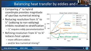
So
this
was
the
major
result
that
we're
able
to
reduce
the
drift
in
in
this
model,
simply
by
using
a
hybrid
vertical
coordinate,
slide.
Six,
just
change
my
view.
So
this
is
remember
that
this
model
was
built
in
the
context
of
a
climate
model
and
and
we
care
very
much
about
drift
and
heat
uptake
in
in
the
climate
system,
which
the
ocean
is
very
much
in
control
of,
and
so
this
is
another
way
of
looking
at
the
previous
result.
So
I'm,
showing
here
the
comparison
again
between
Z
style
and
hybrid,
coordinates.
A
It
is
a
huge
amount
of
heat
being
taken
up
by
the
ocean
and
presumably
because
of
Justice
viewers
mixing
due
to
the
vertical
coordinate,
whereas
the
solid
blue
line
is
the
hybrid
coordinate
model
that
we
used
in
the
final
used
in
the
climate
model,
and
you
can
see
that
the
drift
is
very
much
less.
So
we
were
very
pleased
with
ourselves
that
we'd
actually
been
able
to
build
a
model
with
such
a
little
drift,
at
least
without
experience.
A
But,
however,
as
you
can
see,
there
is
a
real
drift
in
the
ocean
and
we
had
actually,
if
you
in
retrospect,
should
have
actually
been
shooting
to
get
that
drift.
If
we
had
the
physics
right
and
and
using
using
realistic,
forcing
what
we're
showing
here
is
repeat
cycles
of,
in
fact
I'm
using
joa
in
these.
A
A
One
with
respect
to
the
observations,
but
one
thing
about
this
plot
is:
it
tries
to
reveal
how
important
Eddies
are,
if
I,
if
I,
do
look
at
the
the
orange
solid
line,
that's
the
half
degree
model
with
the
parameterized
at
ease
and
if
I
turn
the
parameterizations
off
that
switches
over
to
the
dashed
orange
line,
and
that
change
is
almost
as
large
as
a
spirit
effect.
You
can
see
that
the
Eddies
are
a
huge
heat
uptake
relative
to
you
know
the
relative
of
the
drip
you've
got
to
get
the
Eddies
right.
A
But
despite
the
the
presumption
here
is
that
we're
actually
resolving
them,
Eddie's
better,
which
makes
them
more
efficient,
and
we
may
also
be
reducing
the
what
the
what
remaining
spurious
mixing
there
might
be,
and
in
doing
so,
we've
we've
allowed
the
ocean
to
take
up
less
heat
and
so
clearly
the
blue
lines
and
the
solid
Blue
Line.
The
cylinder
solids
orange
lines
are
somewhat
fortuitous.
A
A
When
you
go
from
half
degree
to
quarter
degree
and
whether
you
know
the
the
benefit
from
going
from
core
two
to
eighth
or
degree
doesn't
appear
to
be
so
obvious.
And
yet
we
saw
that
there
is
a
change
in
in
the
efficiency
of
the
ideas,
as
we
do
that
as
we
go
to
the
next
resolution.
So,
let's
jump
to
the
next
slide,
so
the
next
slide
is
the
one
which
is
slide.
Eight
we're
going
to
move
to
slide
eight.
So
this
is
a
a
result.
A
This
is
something
which
we
haven't
yet
published
and
I
think
it's
extremely
reveals
a
potential
for
for
getting
a
building
a
model
with
with
such
low
drift.
So
this
is
a
comparison
again
of
the
hybrid
vertical
coordinate
between
and
the
Z
coordinate
on.
The
left.
I've
got
the
hybrid
in
the
middle
I
have
the
Z
coordinate,
and
this
is
the
50-year
trend
in
temperature
in
the
top
2000
meters.
A
It's
only
horizontally
average
of
an
inter-annual
core
forced
run
and
the
difference
is
between
the
two
lift
panels
are
I
hope
obvious.
You
know,
there's
some
broad
structures
that
look
very
similar,
there's
big
blue
spots,
but
there's
this
big
warming
in
the
thermocline
around
500
and
below,
and
then,
if
you
compare
that
to
the
right
to
the
right
hand,
panel,
this
is
and
an
estimate
of
the
50-year
change
in
the
real
world.
A
So
if
you
go
to
the
next
slide,
slide
nine
now,
comparing
again
to
the
same
observations,
because
there
is
only
one
set
of
observations,
the
left
hand
side.
What
we've
done
now
is:
we've
switched
from
the
core
forcing
to
the
JRA
55do
data
set
and
now
you'll
see,
there's
a
lot
more
similarity
between
the
model
Trend
and
the
observations
and,
moreover,
I'm
now
showing
an
eighth
of
degree.
Solution
versus
the
quarter.
A
Degree
solution
and
you'll
see
that
there
is
very
little
change
in
this
drift
and
the
blue
spot
has
changed
its
structure,
we're
using
the
hybrid
coordinate
here.
So
we're
not
seeing
this
thermocline
drift
and
you'll
see
I.
Think
to
my
eye,
there's
a
large
similarity.
A
lot
of
the
observational
Trend
seems
to
be
explained
by
this
model,
so
this
is.
This
is
really
really
exciting
because
it
really
helps
it
really.
A
You
know
it
means
that,
for
from
the
point
of
view,
say
data
simulation
and
trying
to
fill
in
the
gaps
in
terms
of
our
observations
using
models,
a
model
with
such
a
little
Drift
actually
looks
like
it
can.
Actually,
you
know,
look
like
the
the
changes
in
the
ocean
can
actually
be
realized,
so
this
is.
This
is
something
we're
very
excited
about,
okay,
so
the
next,
so
so
I've
shown
you
so
far.
A
I've
shown
you
some
very
so
positive
aspects
of
the
model,
but
the
model
is
that,
shall
we
say
far
from
perfect
this,
the
the
input,
the
sort
of
incentive
we
had
to
start
looking
at
hybrid
coordinates,
was,
was
to
try
and
tackle
the
spurious
mixing
problem
and
associated
with
this.
Was
this
idea
that
the
icpigner
models
of
the
previous
generation
were
pretty
good
at
getting
deep
and
strong
amok
circulations?
A
A
We
believe
that
there's
a
mixture
of
physics
as
I'll
show
on
the
next
slide
and
also
choice
of
coordinate,
but
we
don't
know
that
yet
until
we've
actually
managed
to
get
the
aim
up
back
to
where
we
would
like
it
to
be
so
on
the
next.
So
this
is
just
showing
a
Time
series
of
amox,
so
there
is
a
segment
of
periodicity,
but
the
structure
was
unfortunate
in
the
vertical.
A
But
subsequent
changes
were
not
really
say.
We
lost
track
of
the
these
properties
as
in
the
subsequent
changes
and
ended
up.
We
think
mixing
away
some
of
the
Denmark
overflow
water,
with
the
explicit
mixing
we
have
since
then
and
I
haven't,
got
any
results
to
show
this
yet
because
there's
still
ongoing
work.
We've
since
then
fixed
the
configuration
to
have
not
so
so
strong
bottom
boundary
layer
mixing
and
it
does
help
a
little
bit.
But
it's
far
from
enough.
A
So
this
is
still
an
open
issue:
how
to
actually
explain
and
fix
the
depth
of
the
of
amok
in
in
this.
In
this
configuration.
But
we
will
be,
we
are
working
on
it
and
we
will
be
releasing
a
newer
version
of
round
four
when
we,
when
we,
when
we're
done
okay.
So
let
me
just
summarize
so
on
the
next
slide
onto
slide.
12
I'm
done,
hopefully
in
a
short
and
short
enough
amount
of
time.
So
so
we
think
going
for
is
a
step
forward.
A
It's
a
step
forward
for
us
for
tackling
State,
making,
making
statements
and
attacking
tackling
and
modeling
ocean
heat
uptake.
We
acknowledge
that
the
configuration
is
imperfect.
We
made
some
mistakes
in
it.
We
have
issues
that
we
are
trying
to
address
still,
but
nevertheless
it's
something
that's
we
think
is
going
to
be
very
useful
for
at
least
in
the
work.
A
D
A
D
A
D
A
A
So
if
you
mix
a
front-end
temperature
along
an
isopy
normal,
it
doesn't
actually
cause
a
diabetic
transfer
of
heat,
so
so
by
virtue
of
following
isopycles
in
the
interior,
we
don't
have
a
projection
of
that
numerical
mixing
into
the
interior,
but
it
does
nevertheless
smooth
out
gradients.
You
know,
along
along
the
coordinates
that
doesn't
that
argument
of
course
means
that
we
do
have
diaper
mixing
due
to
infection
wherever
we're
using
Z
coordinates
up
in
the
upper
ocean,
but
there's
so
much
mixing
there
anyway.
You
know
the
rationale.
Is
it
doesn't
matter?
A
A
Yes
and
the
goal
is
to
to
be
isoping
all
as
much
as
you
can
be,
but
it's
actually
very
hard
to
construct
this,
and
in
fact
this
is
work,
we're
working
with
Alan,
Warcraft
and
lyric
chasnier
to
try
and
import
their
a
vertical
grid
generator
to
improve
on
what
we
did.
What
we
did
was
a
very
straightforward,
hybridization
and
high
com.
The
hicom
crowd
had
learned
quite
a
long
time
ago
that
you
need
to
be
a
bit
more
sophisticated
than
the
way
we
did
it.
A
So
so
there's
there's,
we
think
room
for
improvement
on
the
court
in
the
coordinate,
Generation
and
we're
finding
when
we
start
we've
had
a
Brandon
weichel,
for
example,
has
been
analyzing,
what's
been
going
on
in
the
operation,
and
we
are
finding
that
there
are
sensitivities
to
how
we
determine
the
vertical
coordinate
at
the
base
of
the
mixed
layer
and
in
the
upper
thermocline.
So
this
is
again
this
is,
you
know,
really
a
work
in
progress.
I
would
say
you
know
there
is
lots
to
be
improved
here.
E
Yeah
Aleister,
as
you
know,
we
have
been
exchanging
about
email,
exchanging
about
these
results,
but
I'm
not
confused
again.
How
do
you
define
your?
What
do
you
mean
by
spurious
because
I
felt,
like
you
are
using
it
both
to
refer
to
numerical
artificial,
spurious
mixing
and
also
improper
and
perhaps
incorrect
representation
of
mesoscale
impacts
in
the
solutions?
Are
you
distinguishing
the
two.
A
Or
I
think
I
think
there's
a
very
good
point
and
perhaps
we
shouldn't
distinguish
I
have
in
my
mind,
we
have
in
our
minds,
thought
about
it
as
spewers
due
to
numerics
but
the
speed.
You
know
whether,
if
you're,
if
you
are
having
some
sort
of
aliasing
effect
or
or
diffusion
due
to
to
Eddie
activity
going
on
at
the
grid
scale,
you
know
it
is
all
spewers.
So
spiritus
might
is
a
very
general
all-encompassing
word
here.
A
Why
well,
or
or
even
perhaps,
mistuned
physics
I
mean
it
could
be,
you've
got
the
right
physics,
but
you
might
have
chosen
so
I
mean
I,
hadn't
I
and
when
I,
when
I
write
the
word
Spirits,
normally
I'm
thinking
about
numerical
only
but
you've,
just
given
me
cover
for
anything,
that's
wrong
with
the
model.
Thank
you.
F
G
C
Fact
I
think
you
almost
say
it's
understood.
One
question
is:
how
does
your
aimog
look
like
in
this
start
simulation
of
quarter
degree,
which
is
very
shallow
in
the
Harvest
coordinate
and
the
second
one
is
I
mean
I
said?
How
do
you
know
if
someone
is
curious?
Is
the
key
between
those
two
heat
uptake?
How
about
your
mission,
or
you
are
very
welcome
to
your
plan
stations
for
the
hibit,
coordinates
and
now
certainly
try
these
start.
It
might
not
work.
A
Yeah
so
well
to
the
latter
question
first,
my
I
think
that
a
good
handle
on
whether
you've,
you've
experienced
in
terms
of
Miss
tuning
can
be
obtained
by
looking
at
sensitivities
to
parameters,
and
we
haven't
yet
found
a
sensitivity
due
to
you
know,
by
changing
a
parameter
that
just
simply
changes
the
depth
of
a
mark.
So
there's
something
else
going
on
here.
A
I
think
the
answer
to
your
first
question
about
comparison
to
Z
Star.
It
was
also
Shadow
and
Z
star,
although
we're
having
to
backtrack
through
our
figures,
to
figure
out
when
this
happened,
because
at
one
point
was
deep
and
we're
trying
to
figure
out
when
that
what
we
know
what's
changed,
we
I
I
mean
I.
We
haven't
put
it
in
the
if
we
didn't
publish
those
results,
but
we
can.
A
H
A
H
Given
that
that
maybe
one
of
the
things
we
as
a
whole
community
and
all
the
people
talking,
could
work
more
on
to
what
kind
of
metrics
and
observation
to
be
trying
to
fit,
and
certainly
Global
measures
like
that
are
not
you
know
going
to
help
us
with
parameter
choices.
You're
gonna
have
to
be
more
Basin,
wide
or
and
I.
Don't
know
what
that
is,
but
that's
another
topic.
We
could
probably
start
to
work
on
even
your.
D
H
H
Yeah
yeah,
yeah,
well
yeah,
cross-eyed,
so
I
think
I
think
maybe
something
we
should
think
about
is
some
of
these
observations
or
metrics
things
we
try
and
and
then
communicate.
What,
when
we
find
sensitivities
like
you
just
mentioned
what
the
heck
is
the
depth
of
the
a
mark
sensitive
to
well,
somebody
might
know
something
here
and
not
over
there.
So
some
idea,
when
we
get
these
metrics
of
communicating
parameters
that
that
have
some
sensitivity
to
that
would
be
maybe
save
a
lot
of
duplication
of
efforts
and
stuff
like
that.
A
G
Oh,
that's
true
I
wanted
to
ask
about
what
we
should
actually
expect
when
we
are
forcing
with
core
or
Jerry
GoGo
in
terms
of
long-term
ocean
heat
uptake,
given
that
these
forcing
data
sets
have
been
purposely
normalized
to
have
zero
net
heat
flux
into
the
ocean
when
coupled
to
observed
SST.
So
if
your
model
was
perfect,
it
should
show
no
net
warming
over
the
time
period
of
the
forcing.
A
Okay.
Well
then,
that
probably
explains
why
we
have
no
drift
in
those
two
when
we
use
those
data
sets
but
yeah.
It's
a
good
question.
So
so
that's
interesting
because
we're
seeing
the
trend
within
the
within
the
60-year
cycle
we're
seeing
the
trend
that
we
want
to
see
as
I
showed
it's
it's
a
challenging
problem.
I
mean
we
don't
have
the
proper
feedback
on
on
the
ocean.
Warming
on
the
fluxes,
so
actually
I,
don't
really
know
Steve.
A
Honestly,
I,
don't
know
how
to
answer
this
I
think
I
I
we've
had
a
repeated
psychic
conversation
at
gftl
and
I.
Think
it's
and
you
know,
spend
a
few
of
you
as
well
about
the
value
in
repeat
cycle.
Forcing
of
the
you
know
in
these
experiments.
You
know
what
happened,
what
does
it
mean
to
run
a
model
that
should
have
Force?
A
You
know
a
heat
uptake
or
a
drift,
and
then
we
setting
it
back
to
the
beginning
if
it
has
indeed
be
been
adjusted
to
have
no
net
forcing
which
I
didn't
appreciate
in
JRA,
then
maybe
that's
more
viable,
but
there
are
still
these
kind
of
discontinuities
and
there
are
Trends
in
the
model
that
we
think
are
real.
So
it's
kind
of
reconciling
that,
with
with
the
idea
that
we
shouldn't
have
any
drift
is
hard
to
hard
to
do
so.
I,
don't
know
how
to
answer
it.
H
Well,
it
goes
back
a
bit
to
Bob's
talk
where
he
said:
there's
no
more
CFL
problem
with
the
in
the
vertical.
So
one
of
the
questions
that
comes
to
mind
is
how
what
is
determining
the
the
highest
resolution
you
can
have
or
your
shallowest
first
level.
Can
it
be
a
meter
half
meter
or
or
what
is
determining
it
now,
because
if
we
start
to
work
on
that
problem,
one
could
conceivably
start
to
get
ssts
that
are
more
like
ssts,
and
it
might
be
something
to
to
think
about
how.
I
We
assume
that
there's
no
feedback
of
the
surface
heat
fluxes
on
the
surface
properties
over
the
course
of
a
Time
step,
and
so,
if
you
take
a
a
piston
velocity,
basically
a
linearization
of
your
of
your
bulk
formula
or,
however,
you
want
to
get
at
times
a
coupling
time
step.
That
says,
your
vertical
resolution
has
to
be
something
of
order:
half
a
meter.
I
H
So
that
would
get
you
most
of
the
way
there
and
I
think
would
would
might
be
something
to
think
about.
With
the
with
the
vertical
coordinate
the
elk
or
the
the
the
layer
coordinate,
get
into
trouble
if
it's
so
thin
that
it
goes
unstable
because,
right
at
the
surface,
you
you're
unstable
right
you're,
if
you're
cooling,
so
would
that
be
a,
but
that's
pretty
fine.
So
is
that
what
would
ultimately
stop
you?
Or
can
you
have
ins
in
unstable
layers.
I
I
Equations,
you
would
also
want
to
make
sure
that
you
have
parametrizations
that
are
able
to
adjust
and
and
kind
of
work.
Implicitly,
that's
one
of
the
things
I
like
about
the
the
Jackson
at
all
scheme
is
it's
kind
of
an
iterative
and
implicit
solver.
If
you
took
the
initial
instability
sharing
stabilities
in
the
surface
and
treated
them
explicitly,
it's
possible
that
that
could
give
you
troubles,
but
I
I,
don't
have
experience
with
with
that
directly.
So
I
seems
to
be
pretty
robust
to
very
fine
resolutions,
so.
A
Just
to
summarize
I
mean
so
there
is
a
problem
with
resolution
at
the
surface
due
to
the
couple
due
to
the
missing
the
way
that
fluxes
are
done,
but
in
interior
we
can
handle
very,
very
thin
layers
and
stably
so
away
from
the
forcing
we
know
we
go
to
submillimeter
regularly.
So
so
there's
no.
There
is
no
no
lower
limit
if
it
wasn't
for
the
forcing.
H
F
I
I
yeah
I
just
had
a
question
a
couple
of
questions
for
Bob
the
first.
You
talked
about
the
need
to
do
additional
pseudocompressibility
passes,
I
think
on
kind
of
a
regional
basis.
I
was
wondering
if
that
needed,
to
be
recalibrated
potentially
for
other
climates,
or
you
know
certain
applications
of
the
model
and
then
the
second
question
is
about
what
tools
are
available
to
accelerate
the
equilibration
of
the
model.
For
instance,
Tracer
distribution.
C
I
So
the
the
first
one,
no
the
model
keeps
track
of
how
much
mass
has
been
able
to
move
from
one
cell
to
another
and
if
there's
more
mass,
to
be
moved,
there's
a
basically
it
keeps
track
of
when
it
needs
to
do
another
pass.
The
number
of
passes
that
you
need
to
do
is
is
kind
of
capped
at
the
number
of
Bearer
Clinic
Dynamics
steps
right.
I
I
I
The
way
we've
done
it
is
we've
just
run
a
long
time,
so
we
would
be
delighted
if
somebody
could
suggest
things
that
work
better,
but
the
other
part
of
it
and
I
think
this
is
going
back
to
alistair's
slides
where,
if
you
start
off
with
the
model
with
less
drift,
even
though
the
intrinsic
e-folding
time
scales
of
the
Water
Mass
property
are
the
same.
If
you
start
off
closer,
you
have
to
go
through
fewer
of
those
e-folding
time
scales
to
before
you
get
to
within
your
tolerance
of
an
acceptable
drift
rate.
I
I
I,
don't
think
it
does,
because
I
think
that
the
Tracer
diffusion
is
dominated
by
the
along
layer.
Mixing
the
effective
mixing
I
mean
I
know
that
some
people
have
done
things
like
in
in
Nemo,
they'll
have
a
z-like
model
and
they'll,
let
it
bounce
up
and
down,
because
they
think
a
lot
of
the
invection.
The
spherus
mixing
is
set
by
vertical
advection
associated
with
gravity
waves.
I
We
do
tend
to
try
to
restore
boards
if
it's
a
z,
light
coordinate
near
the
surface,
we'd
like
to
kind
of
keep
the
time
scale
shorter
than
about
a
day,
because
I
think
that
the
diurnal
cycle
and
could
give
you
some
kind
of
weird
aliasing.
If
you
have
Ekman
pumping,
that's
driving
your
your
top
layers
resolution
deeper
over
the
course
of
of
a
day
or
something
that
would
be
a
bit
weird.
We've.
Never
really
explored
whether
you
could
how
far
you
can
push
it,
but
that
would
be
an
interesting
study.