►
From YouTube: Robert Helber Regional MOM6 for the Nordic Seas
Description
No description was provided for this meeting.
If this is YOUR meeting, an easy way to fix this is to add a description to your video, wherever mtngs.io found it (probably YouTube).
A
Full
screen
there
you
go.
Thank
you:
I'm
Bob,
helber
I
work
at
the
naval
research
lab
and
we
are
using
mom
6
in
the
Nordic
Seas
for
a
project
that
I
have.
So
what
I
want
to
do
is
just
say
what
the
objectives
of
the
project
are
and
why
I
think
Mom
six
will
be
a
useful
tool
and,
and
some
very
preliminary
results
that
we
have
using
the
model.
A
A
Can't
okay
good,
so
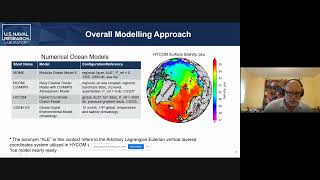
this
is
High
Comm,
which
is
one
which
is
our
Global
model
that
the
Navy
uses
for
forecasting.
This
is
sea,
surface
salinity,
and
so
these
warmer
saltier
waters
are
moving
further
up
into
this
region
of
the
ocean
and
it's
changing
the
circulation.
And
so
what
we
want
to
understand
is
is
how
it's
changing
in
detail.
A
A
So
you
have
the
warm
salty
Waters
flowing
flowing
North
and
then,
when
they
get
up
in
the
green,
let's
see,
there's
deep
convection
and
then,
if
it
goes
up
into
the
into
the
Arctic,
it
goes
beneath
the
colder
water,
creating
the
halocon
and
then
when
these
waters
are
created,
they
flow
back
over
through
through
particularly
the
Denmark
Strait.
So
these
These
are
the
water
mass
changes
that
we're
interested
in
in
understanding
how
they're
changing
and
how
they're
affecting
the
circulation
Dynamics.
So
that's.
A
So
those
are
the
kind
of
questions
that
we're
trying
to
answer
with
this
modeling
study
and
I.
Think
Mom
six
could
help
us
with
that,
so
more
about
the
Deep
convection,
so
in
the
Greenland
sea.
Traditionally,
the
Greenland
sea
gyre
is
where
there
would
be
deep
convection.
This
is
the
Symmetry
I'm
showing
on
the
left
there's
an
interesting
paper
in
2018,
where
they,
where
they
published.
You
know
Decades
of
temperature
data
from
the
middle
of
the
Greenland
sea
and
so
like
in
the
90s.
A
You
would
see
these
these
this
deep
subsurface
temperature
maximum,
which
is
a
signature
of
deep
convection
I,
would
go
very
deep
there
and
but
it
doesn't
seem
to
be
occurring
anymore,
so
suggesting
that
the
circulation
and
Greenland
Seas
is
changing.
The
convection
has
gone
elsewhere.
So
the
question
is:
where
is
the
convection
occurring
now?
How
is
the
deep
water
forming?
A
So
those
are
the
kind
of
questions.
So
one
reason
that
I'm
pointing
this
out,
which
is
relevant
to
modeling,
with
with
isopycno
coordinate
model,
is
that
particularly
in
the
90s.
You
would
have
these
situations
where
you
would
have
an
inversion
in
Sigma
2..
So
what
I
mean
by
that
is
Sigma
2?
What
I'm
saying
here
is
actually
a
density
potential
density
reference
to
2000
decibars
minus
one
thousand,
so
that's
where
the
sigma
comes
from
that's
different
from
the
coordinate
Sigma,
which
I'll
be
I'll
mention
later
so
anyway.
A
This
is
a
row
two
there's
an
inversion
that
occurred
a
lot
back
here
in
the
90s.
So
the
reason
this
is
important
is
if
your
model
like
high
com
or
mom6-
and
you
have
Sigma
2,
coordinates.
Then
you'd
have
an
inversion
here
and
what
happens?
Is
we
ran
a
test
with
this
with
high
competent
melee
mixes?
All
of
this
out?
So
it's
unrealistic,
so
you
don't
want
that.
A
So
we're
being
real,
careful
to
take
a
look
at
our
model
runs
to
make
sure
that
if
we're
using
Sigma
2
coordinates
we're
not
having
a
problem
with
these.
These
big
inversions,
which
can
go
down
to
500
meters,
that's
one
thing:
we
have
to
keep
take
into
account
when
we're
using
a
model.
The
kind
of
questions
we
want
to
experiments
we
want
to
run
are
understanding
the
circulation
Dynamics
associated
with
the
the
receding
of
the
sea
ice
in
and
at
high
latitude.
A
So,
for
example,
this
is
from
the
Ice
Center
on
the
left
is
a
March
1998
and
you
can
see
there's
a
lot
of
ice
in
the
green.
Let's
see,
there's
a
tongue
of
ice
in
there,
that's
not
doesn't
occur
nearly
as
much
in
2018,
so
this
would
suggest
a
different
current
structure,
and
so
what
do
we
need
to?
What?
A
How
are
we
going
to
model
this
more
accurately
in
our
models
want
to
quantify
the
difference
in
the
circulation?
How
do
the
current
structures
change
based
on
this,
on
the
changing
sea
ice
conditions
and
how?
How
best?
What
kind
of
model
do
we
need
to
represent
this?
This
circulation
as
as
well
as
possible?
A
There
were
some
interesting
observations
made
in
2018.
So,
first
of
all,
if
you
look
on
the
left
here,
I've
got
a
satellite
SAR
image
and
you
can
see
that
the
sea
ice
has
got
a
lot
of
structure
along
the
edge
there's.
A
lot
of
you
know,
Eddies
and
submissive
scale
features
in
the
ice
itself.
So
it's
not
just
a
straight
thing,
but
our
sea
ice
model,
which
here
is
probably
C
ice4
version
4
here,
maybe
that
we're
using
operationally
and
it's
it
doesn't
have
all
this
structure.
A
It
doesn't
have
this
this
fine
scale
structure.
So
what
is
the
impact
of
that
on
the
circulation?
We
know
that
that
these
do
have
impact,
because
in
2018,
Bob,
picardo
Tui
went
out
in
the
RV
Alliance
and
I
actually
drove
out
right
along
here
into
the
ice
and
we're
taking
measurements.
So
the
color
is
potential
temperature
and
these
lines
are
potential
density
reference
to
the
surface
minus
a
thousand,
and
so
there
was
sea
ice
over
here.
A
There
was
sea
ice
cover
when
he
drove
into
the
eyes,
and
so
you
get
this
cool
polar
water
which
is
associated,
which
can
exist
only
because
of
the
sea
ice
and
then
there's
varying
Ice
concentrations
out
here
associated
with
these
different
subsurface
features.
So
I
would
suggest
that
a
lot
that
this
does
have
a
big
impact
on
the
circulation
and
how
does
that
affect
the
the
current
structure
along
here?
The
dissipation,
the
kinetic
energy
things
like
that.
So
these
are
the
kind
of
questions
we're
trying
to
answer
and
I'm.
A
I
forgot
to
mention
that
NRL
traditionally
had
spent
a
lot
of
time
on
the
sea
ice
modeling,
but
this
project
is
is
to
look
down
deep,
so
we're
more
interested
in
the
subsurface,
so
got
a
modeling
project
which
includes
mom
six,
which
is
why
I'm
here
talking
and
so
the
models
we
have
are
our
mom
six.
Of
course
we're
interested
in
that
because
of
it's
a
it's
an
ale
model,
meaning
that
the
the
coordinates
literally
move
with
with
the
with
the
water
masses.
A
It's
a
arbitrary
LaGrange
eulerian
coordinates,
of
course,
we're
interested
in
that
capability.
So
in
everything
we've
done
here,
we're
using
the
high
Comm
1
coordinates
that
we
saw
earlier
today
and
hopefully
we're
we're
thinking
right
off
the
bat
that
that's
what
we
need,
because
we're
used
to
using
that
in
high
Comm.
A
So
we
think
that
that's
the
coordinates
that
we
want
to
make
so
we're
gonna
we're
gonna,
we're
gonna,
look
at
those
we
may
need
to
step
back
and
and
look
at
maybe
Z
Star
coordinates
if
if
this
isn't
working
right,
but
the
idea
right
away
was
that
we
wanted
to
use
the
high
Comm
1
coordinates.
Hopefully,
maybe
that'll
pan
out
we'll
see
the
model
that
we
we
do.
A
lot
of
work
with
at
NRL
is
ncom,
which
is
a
Navy
Coastal
ocean
model.
A
So
I'll
show
you
a
little
results
from
that
today
and
the
interesting
thing
about
that
is
that
we've
got
income
and
it
runs
with
our
co-amps
atmospheric
model,
and
this
is
a
tightly
coupled
system
I'm
going
to
talk
a
little
bit
more
about
that
in
the
next
slide,
where
we
actually
couple
it
with
with
the
model.
So
we
have
Internet.
We
have
our
own
coupling
system.
A
Ncom
is
a
sigma
Z
level
model,
so
it
doesn't
have
the
ale
capability,
it's
an
older
model.
So
it's
a
it
does
have
tides
for
the
bear:
Tropic
tides
at
the
boundaries.
It's
it's
Sigma
zero,
but
it's
a
z
level,
fixed
coordinate
model
so
that
I
don't
think
the
inversion
in
Sigma
2
is
a
problem.
With
this
model.
A
A
A
We
also
have
a
Global
digital
environmental
model,
which
is
a
climatology
that
we
use
at
NRL
version.
Four
is
about
10
years
old.
We
just
are
redoing
our
model,
so
we're
gonna
have
an
updated
climatology,
so
I
want
our
initialization
of
our
model
is
going
to
be
more
more
relevant
to
the
changing
conditions
with
our
new
climatology.
A
So
what
so?
Oh
yeah
right,
I
forgot
I
wanted
to
tell
you
about
the
the
co-amp
system.
It's
it's
a
tightly
coupled
system.
Typically,
we
couple
every
six
minutes,
Between
the
Ocean
and
the
atmosphere,
and
and
then
we
have
the
the
co-amp's
atmospheric
model.
So
it's
a
model
that
that
runs
along
with
the
income.
A
So
we
want
to.
We
want
to
take
a
look
at
the
impact
of
cold
air
outbreaks.
That's
at
the
flow
like
particularly
through
the
Denmark
Strait
over
here
on
the
right
is
sea.
Surface
temperature
from
that
model-
and
here
is
the
little
black
line-
is
this
transect
here?
So
this
is
ncom
and
with
the
barrel,
barotropic
tides.
A
This
is
2014.
over
here.
Just
just
for
comparison.
We've
got
high
com
with
the
zonal
velocity.
This
has
this
was
a
non-assembling
overrun
with
a
full
title
model.
So
it's
not
greatest
comparison,
but
just
for
example,
just
a
show
you
what
these
these
models
can
do.
We
have
them
running
in
NRL.
So
the
main
point:
what
I
wanted
to
show
was
was
a
twin
experiment,
we're
working
on
between
mom
6
and
ncom
and
the
Nordic
Seas.
So
the
resolution,
it's
just
a
regular
grid,
regular
square
grid,
so
it's
not
curvilinear.
A
So
what
it
means
is
down
here.
We've
got
for
about
four
and
a
half
kilometers
up
here.
It's
about
one
and
a
half
kilometers.
This
is
a
bathymetry
over
here
on
the
right
I'm,
just
showing
the
the
Delta
X
horizontal
grid
on
the
H
grid,
so
we're
we're
running
for
both
mom
6
and
ncom
800,
one
by
485
grid
points.
Right
now.
We've
got
Mom
six
running
at
41
layers
and
end
com
at
100,
Sigma,
Z
levels.
A
We've
got
right
now:
we've
got
different,
forcing
mom
six
has
got
nset
reanalysis
forcing
and
ncom
has
got
the
US
Navy
navs
gem,
so
we
wanna
make
them
both
use
nav
gems.
But
at
this
point
we
don't
have
that
we're
still
getting
our
ducks
on
a
row.
The
the
boundary
condition
is
a
global
High,
Comm
and
an
initialization
is
is
another
difference.
I
think
Mom
six
is
initialized
from
acclimatology,
where
income
is
initialized
from
the
global
ocean
forecasting
system,
so
I
just
have
just
very
brief
results
of
this.
A
So
what
we
have
here
is
a
Surface
salinity
on
the
left
is
is
Mob
six.
This
is
just
for
nine
days,
we're
running
it
longer
on
HPC.
Maybe
our
performance,
Computing
Center,
we
don't
I,
don't
have
the
results
to
show
just
yet
there's
a
few
things
we
need
to
fix
before
we
do
any
real
long
runs
and
on
the
right
is
end
com
salinity
at
the
surface.
This
is
just
the
full
month
of
January.
A
If,
if
we
need
to
block
out
some
grid
points,
that
Kate
was
just
telling
us
about
I'm,
not
sure
we
have
that
correct
yet
so
we
we
may
need
to
take
a
closer
look,
because
I
just
learned
that,
just
today
what
Kate
was
telling
us
about
the
about
the
boundary
conditions
near
the
edge
of
your
of
your
condition.
So
we
may
need
to
take
a
look
at
that.
Oh
yeah
up
here.
Maybe
we
need
to
do
that,
so
so
there's
some
more
work.
A
So
it's
going
to
be
very
interesting
to
see
how
these
models
model
this
section
of
the
ocean,
so
right
off
the
back.
Looking
at
the
end
com,
you
see
this
Jagged
topography,
there's
a
couple
things
going
on
here.
First
of
all,
the
we
ran
this
with
100
layers,
but
the
post-processing
net
CDF
files
only
have
40
layers,
so
we
need
to
go
back
and
reprocess
that,
but
rather
I'm
going
to
plot
the
sigma
layers,
because
this
model
is
Sigma
Z,
so
it
would
be
Z
levels
out
here
in
Sigma
along
the
coast.
A
So
I
need
to
plot
that
in
detail.
So
there's
a
little
more
work.
We
need
to
do
on
ncom,
but
mostly
with
the
output
I
think
the
system
seems
to
be
running.
It's
a
pretty
stable
system,
we've
run
for
a
while,
although
we
haven't
run
this
income
co-amps
at
high
latitude
very
much.
So
it's
a
little
we're
a
little
new
in
this
this
domain.
A
This
is
a
new
domain
for
us
to
run,
and
maybe
we
need
to
we're
still
we're
still
working
on
how
to
get
this
just
right.
So
what
I
have
here
is
on
the
left
is
the
mom6
for
the
same
nine
days
and
there's
a
few
things
here.
First
of
all,
what
I'm
plotting
is
the
the
temperature
in
every
little
grid
box
is
what
the
colors
are
are
a
little
patches
in
the
in
the
per
the
grid
grid
for
every
grid
cell.
A
That's
a
little
patch,
which
is
the
temperature
in
that
that
grid
cell
I
just
and
the
and
the
lines
are
the
the
interface
is
depths
that
are
coming
out
of
of
of
mom
six
and
it's
it's
interesting
that
they
follow
the
follow
the
water
masses,
which
is
what
we
want,
which
I
think
we
why
we
need
a
layer
model
that
operates
like
this,
an
ale
model,
which
is
why
we
would
really
like
to
be
using
this
High
Comm
1,
coordinate
system.
There's
one
problem
here:
I
guess
this
would
be.
A
We
didn't
have
the
right
target
densities
to
extend
these
layers
into
this
region
of
the
ocean.
It
turns
out
that
you
have
to
because
I
knew
this,
but
we
we
didn't
select
the
densities
light
enough
to
go
to
fill
this
Gap
so
that
there's,
there's
I,
think
14
layers
up
here
that
are
Z
level.
What
those
are
are
Target,
densities
that
are
very
light
and
those
are
designed
to
be
light
so
that
you
always
have
a
surface
a
z-level
region
in
the
model.
A
The
problem
is
our
first
density
layer
wasn't
light
enough,
so
we
have
this
big
gap
here.
So
I
need
to
go
back
and
and
redo
that
another
thing
traditionally,
these
Target
densities
are
chosen
as
exponential
decay,
so
they
would
get
more
coarse
down
here,
but
I
don't
really
want
to
do
that.
I
want
to
have
a
lot
of
layers
going
through
here.
So
I
chose
a
linear
array
of
Target
densities,
which
is
traditionally
not
done.
A
A
We've
got
mom6
running
at
NRL
and
sip
Force,
the
Nordic
Seas,
the
boundary
conditions
are
high
com,
Global
ocean
forecasting
system
over
comparing
it
with
our
income
model
and
we're
we're
adjusting
the
target
densities
to
make
it
work
appropriately
in
the
Nordic
Seas,
and
we're
also
potentially
going
to
change
the
densities
to
surface
reference
density.
Excuse
me
the
Target,
the
coordinates
to
surface
rest,
reference
density
rather
than
Sigma
2,
because
in
the
Arctic,
Ocean
or
high
latitude
you
may
have
those
inversions
and
we're
also
we
are
going
to
do
ice.
B
A
Yeah,
so
this
this
has
to
do
with
the
compressibility
in
in
in
the
coordinate
system,
so
it
for
Regions
that
are
that
are
highly
unstratified.
There
is
a
an
option
to
add
a
little
compressibility
so
that
you
have
you
actually
have
a
stratification.
So
this
the
option
here
the
progressibility
was
.01,
which
was
the
option
which
was
like
a
default
option
in
there.
That
is
one
of
the
things
we
we
may
need
to
adjust.
A
I
got
some
advice
from
the
regional
modeling
group
last
week
that
we
may
need
to
adjust
that
so
yeah.
So
this
is
a
region,
that's
got
low
stratification
and
that's
why
they
were.
They
were
Z
level,
although
it
seems
seemed
like
there
was
more
stratification
here,
so
we
we
do
need
to
address
this.
A
little
more
I'm,
not
exactly
sure
why
these
are
so
straight
here,
we'll
adjust
the
compressibility
parameter
and
see
if
see.
If
this
will
will
change
things
but
yeah
that
is
that
is.
A
B
B
C
So
it
was
a
good
question
that
you
asked
Frank
so
in
in
the
the
high
com
mode,
you
specify
the
density
and
it's
mostly
Sigma
2,
as
Bob
said,
although
we
can
put
in
a
little
bit
of
compressibility.
So
you
have
some
resolution
where
there's
stratification,
but
each
layer
is
also
given
a
minimum
depth
from
the
surface
at
which
you'll
find
it
and
when
the
water
is,
is
really
dense.
C
That,
in
fact,
it's
denser
than
the
target
density
of
a
layer,
then
each
of
the
layers
tracks
that
specified
minimum
depth
at
each
of
the
interfaces
follows
the
minimum
minimum
depth.
So
it
really
is
a
z
coordinate
there
for
those
layers
whose
Target
densities
are
lighter
than
anything
in
the
water
column.