►
From YouTube: 2023 Atmosphere Model WWG- Day 3 AM Session
Description
No description was provided for this meeting.
If this is YOUR meeting, an easy way to fix this is to add a description to your video, wherever mtngs.io found it (probably YouTube).
B
B
B
Indoor
Global
models,
and
why
do
we
need
to
move
on
from
the
lookup
table
approach
we've
been
using
for
quite
a
while
and
then
show
some
first
results,
just
comparing
catalysis
race
of
tubx,
inline
and
csm2
versus
the
lookup
table
and
then
taught
briefly
about
our
spatial
means
for
LACMA
Matt,
Dawson's,
probably
online.
And
if
you
have
any
like
detailed,
you
know
and
system
kind
of
questions
about
tudx
you
can
certain
Agents
from,
but.
B
Slide
and
it
basically
the
reason
they
started
with
Sasha
madronich's
TUV
5.3,
and
they
just
basically
tore
it
apart
and
put
it
back
together
and
they
brought
it
up
to
more.
Modern
programming
techniques
is
more
portable.
It
builds
as
a
software
Line
library.
So
once
it's
built
you
can
you
can
link
it
to
any
application.
It's
configurable
a.
B
B
B
So
this
is
just
the
example
that
information
has
been
put
in
these
Json
files
and
on
the
right
are
cross
sections
and
Quantum
yields,
and
so,
if
it's
a
simple
reaction,
that's
you
know
a
molecule.
That's
already
in
the
database.
You
could
play
around
with.
You
could
switch
it
in
or
out
and
it
has
complicated
temperature
dependence
and
pressure
dependence
and
you
have
to
go
into
the
source
code.
B
If
you
want
to
learn
more
about
tuvx
I
asked
Matt
to
put
this
together,
you
can
go
to
a
GitHub
site
and
it's
listed
here
so
just
download
this
presentation.
You'll
have
all
this
information.
It
runs
in
a
docker
program
and
I'll.
Let
Dan
Marsh
talk
about
that
if
he
wants,
but
you
know
so,
you
should
be
able
to
run
it.
You
know,
run
it
download
it
even
Orlando.
Can
you
know
probably
get
it
going
so.
B
B
B
D
B
Have
to
figure
out
how
we're
going
to
manage
this
there'll,
be
something
like
what
reasons
don't
nicely
with
the
chemistry
Cafe.
So
we're
certainly
open
for
comments
on
this
and
how
to
move
forward.
Tuvx,
of
course,
had
can
have
multiple
radio
transfer
choices
from
two
streams:
X
string,
32
stream.
You.
B
You
got
to
be
careful
because
it's
going
to
cost
a
lot
of
money
from
computer
time
to
to
run
again
the
radio
transfer
it
is
I,
don't
know
what
this
Arrow
looks
so
yeah.
The
radio
transfer
now
can
have
aerosol
and
clouds,
but
any
constituent
since
and
Chuck
has
a
version
of
tub
in
CSM
too,
and
he's
he's
really
done
a
nice
job
of
playing
around
with
this
and
I'll
mention
that
later
saucer
padronic
has
something
called
the
web
base.
Quick
t!
U
v
and
I'll
show
example
of
that.
B
That's
the
Standalone
profile
that
you
can
run
music
box.
So
this
this
version,
the
TUV,
will
run
the
Box
model
and
Luisa
talks
a
little
bit
about
that
from
the
mickum
presentation
she
gave
earlier,
and
then
this
version
of
TUV
also
support
the
aircraft
campaign
s
cast
and
harp
instrument
that
makes
us
tinting
flux.
B
B
This
is
the
TUV
webpage.
It's
important
to
keep
this
going.
So
if
you
would
like
that,
it's
you
know,
since
2016,
it's
been
over,
231
000
hits
on
this
page
and
deriving
catalysis
rates.
If
you,
if
you
look
at
the
harps
calf,
Airborne
attending
flux
measurements,
so
they
use
this
in
the
field
they
take
TV,
they
measure
attending
flux.
They
put
that
into
tub
use
across
and
a
given
set
of
cross-sectional
Quantum
yields,
for
example,
for
NO2,
and
they
calculated
J
rate.
B
Then
they
run
TV
clear
sky
without
that
attending
blocks,
and
that
tells
them
a
lot
about
where
they're,
at
where
the
clouds
are
at,
if
they're
flying
above
the
clouds
or
below
open
clouds
and
that's
what
this
figure
on
the
right
is
showing
here.
This
is
a
ratio
of
the
measurements
to
the
clear
sky
TV.
There.
B
Of
other
things
that
they
do
with
this
model,
but
that's
another
reason
to
keep
the
database
available
in
the
code
moving
forward
so
that
a
lot
of
people
can
use
it
so
Global
modeling.
What
are
the
needs?
Well,
several
people
in
this
room
have
been
working
on
versions
of
or
science,
topics
that
require
aerosols,
sulfonator
soot,
Simone
has
worked
in
geoengineering
and.
B
Is
you
know
these
inputs
of
sulfate
or
Center
going
into
the
radio
transfer
so
and
that's
something
I
know
that
she
really
wants,
and
it's
really
important
for
volcanic
eruptions.
Susan
Solomon
works
on
wildfires
and
you
know
organic
aerosols
get
into
the
stratosphere
if
you'd
like
to
have
that
affect
the
radiative
component
and
the
photolysis
rates
early
atmosphere,
stuff,
Dan,
Mars
has
been
working
on
or
O2
and
O3
are
low.
This
is
probably
going
to
be
very
useful
for
that.
You
know.
Clouds
would
be
different
in
an
earlier.
B
If
you
know
it'd
be
nice
to
know
how
that's
affected
asteroid
impacts.
Garcia
bardine
have
destroyed
the
world
several
times.
Looking
at
this
topic,
they
injected
soot
water,
knocks
halogens
Etc,
and
then
the
nuclear
war
scenarios
were
against
soot,
organic
Aeros
cells
could
be
ejected,
not
will
be
elevated,
and
so
all
these.
E
D
B
This
is
the
first
result
and
believe
me
this.
These
look
really
good
compared
to
the
very
first
results,
yeah
that
we
were
looking
at
this
weekend
and
and
thanks
to
Matt
he
he
made
these
last.
These
plots
for
me
yesterday
about
five
o'clock
so
on
the
left
is
j02
going
to
two
o
triple
p
and
the
kind
of
goldish
line
is
the
lookup
table
and
the
blue
line
is
cuvx.
There
are
some
differences
here,
and
these
are
pretty
large
differences
on
the
log
scale
here.
B
Photolysis,
both
branches
I'm
only
showing
one
here
right
on
so
it
looks
like
from
the
tinting
flux
on
down
the
lookup
table
and
tubx
are
doing
really
well.
If
you
go
to
another
species
methyl
hydroperoxide,
this
species
has
cross
sections
between
210
and
365
nanometers.
It
doesn't
have
any
temperature
dependence
pressure.
Independence
I
picked
this
because
I
just
want
to
see
what
it
looks
like
and
assuming
that
we're
using
the
same
cross
sections,
which
I
think
we
are
there's
some
differences,
but
not
a
lot.
B
So
maybe
this
is
some
radio
transfer
differences,
I,
don't
know,
but
based
on
this
ozone
comparison
I
doubt
that
so
I'm
a
little
confused,
light's
different
nitrogen
dioxide
here
is
another
one.
That's
a
little
different
up
high.
This
is
a
linear
scale.
So
it's
not
a
huge
error,
but
this
is
probably
due
to
the
temperature
depends
the
nitrogen
dioxide
and
that's
something
we
can
check.
So
you
know
from
my
point
of
view,
this
was
pretty
exciting,
because
now
we
have
something
that's
wrongable.
We
can
get
into
the
guts
of
it.
B
G
B
Yeah
I'm
sorry
I
didn't
say
that
this
is
the
launch.
So
it's
a
point
in
the
tropics
at
0.47
degrees
and
it's
a
sonal
average
and
then
the
bars
or
the
deviation
alone,
so
that
could
just
be
clouds
causing
that
shift.
So
probably
not
probably
not
in
the
stratosphere.
You
know
yeah.
These
are
runs
simultaneously,
so
it
should
be
looking
at
the
same
clouds,
but
that's
the
probosphere.
H
D
D
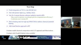
B
Actually
really
fun
and
then,
finally,
you
know
the
special
needs
model.
Wacom
is
going
to
have
to
calculate
the
heating
rates,
the
this
from
solar
energy,
the
solar
energy
energy
beating
rates.
Essentially,
as
we
derived
the
photolysis
rates
for
j02
j07,
we
have
to
subtract
off
the
bond
dissociation
energy,
because
all
that
energy
of
that
Photon,
hitting
the
molecule
in
the
mesosphere
and
water
thermosphere
isn't
realized.
Products
can
go
in
other
places
and
come
back
together,
react
and
release
exothermic
energy
heat
and.
H
B
I
B
If
you
can,
if
you
can
help
he's
had
a
lot
of
experience
and
and
Matt
and
Stacy
have
already
kind
of
got
a
template
set
up
to
do
that,
we're
going
to
start
testing
the
costs
of
the
four
string
versus
the
two
string
and
see
if
we
have
to
minimize
wavelengths
a
little
bit
in
the
in
the
visible,
hopefully
not
I,
don't
really
want
to
go
down
that
fast
shape.
Half
I'd
like
to
just
use
the
computer
power
to
do
the
The
Little
J.
B
We
have
to
drive
between
races,
I
just
said
from
a
chemical
potential
Heating
and
then
come
up
with
the
cloud
traction
approach
for
the
radio
transfer
and
there's
some
options
out
there.
But
that's
what
I
got
and
so
I'm
really
hopeful
by
the
time
the
next
working
group
meeting
comes.
This
is
going
to
be
it'll,
be
you
know
in
inline,
a
csm2
or
whatever
version
of
the
model.
We
have
to
go.
B
G
Time
for
a
couple
questions
there
yeah,
so
we
need
the
plan
that
will
be
up
to
keep
the
lookup
table
in
there,
as
well
as
an
option.
I
would
suggest
what
I
was
thinking
is
that
it
would
be
great
if
this
code
could
be
run
for
whatever
Earth
you
want,
and
it
would
then
be
able
to
Output
a
lookup
table
that
could
be
read
in
so
you
could
do
it
right,
create
a
table
for
a
particular
atmosphere,
Act
through
a
short
run
a
year
long
or
whatever.
B
B
A
A
I
Nitrogen
sources
in
the
upper
troposphere
during
the
Asian
Summer
monsoon-
this
is
a
very
preliminary
and
in
Progressive
study,
but
I
think
it
would
be
very
existing
to
show
here.
First
I
would
like
to
acknowledge
all
my
co-workers
and
for
their
tremendous
help
and
support
and
okay.
So
why
do
we
want
to
study
marks
in
the
other
service
there?
So
previous
study
have
shown
that
there
is
nox
anomaly
over
the
Asian
Summer
monsoon
region.
I
So
don't
know
this
at
all
in
2015
contact
the
transport
of
emissions
to
the
upper
charter
school
is
the
largest
factor
affected
amongst
there,
but
laterally
at
all
times
that
likelihood
and
skill
of
Peace
source
of
knocks
in
the
architectural
Square
motion
region.
So
the
Knox
play
a
critical
role
in
the
chemistry
in
the
upper
tractor.
I
So
what
could
be
the
long
sources
in
the
architecture
sphere
within
the
monsoon
region?
First,
we
would
have
the
surface
emissions,
including
a
supergenic,
biomass,
burning
and
soil,
and
among
them,
as
object,
is
the
biggest
Factor
and
I
also
have
lightning
can
produce
Knox
associated
with
deep
convection,
and
you
also
have
air
product
approximation
within
the
stratosphere.
Nitrous
oxide
can
undergo
fatalities,
produce
Max,
which
can
also
transport
into
the
uppercut
sphere.
I
Okay.
How
do
we
attack
knots
in
the
chemistry
mechanism?
All
the
sources
are
considered
simultaneously,
but
each
natural
limited
is
characterized
by
an
artificial
treasure.
X
Knox,
so
example
here
shows
that
x
max
species
are
added
for
each
reactions
related
for
species
like
n2o5.
There
are
three
Pathways
that
can
form
tax
into
a
fire
and
they
are
all
added
to
the
mechanism
for
detailed
mechanism.
I
Please
look
at
the
research
paper,
so
this
mechanism
allowed
us
to
follow
the
evolution
of
nitrogen
from
each
source
and
regions
without
affecting
the
overall
chemical
system
of
atmosphere
compared
to
the
traditional
commonly
used
technique.
Perturbing
Knox
emissions
like
by
20.
You
know,
region
to
determine
its
impact.
This
technique
can
have
the
advantage
of
eliminating
the
long
immunity
induced
to
the
chemistry
okay.
So
we
use
the
welcome
6
110
level
for
the
Target
study.
It
has
a
horizontal
resolution
of
one
degree
and
vertical
revolution
of
500
in
the
udrs
region.
I
I
Okay.
So
let's
look
at
the
Knox
sources
in
the
monsoon
region
first,
so
the
pie
graph
here
shows
that
the
Knox
sources
from
five
simulations
and
derived
stratospheric
contributions
and
the
blue.
The
blues-
are
the
contributions
from
South
Asia.
With
the
light
color
devotes
the
south
Asia
as
periodic,
and
the
darker
color
is
the
lightning
okay.
So
the
orange
yellow
color
shows
the
configuration
from
East
Asia,
with
the
lighter
color
from
esophagenic
same
as
South
Asia
and
the
darker
color
lightline
source,
and
the
gray.
I
So
we
can
see
that
within
the
monsoon
region,
the
south
Asia
sources,
including
the
natural
progenic
and
lightning,
are
the
major
Knox
sources
account
for
about
60.
What
is
the,
what
are
the
East?
Asia
sources
become
more
significant
in
the
sharing
region,
which
is
40
percent
more
than
the
contribution
from
South
Asia.
I
Okay,
now
we
are
looking
at
I,
don't
know
to
oh
production
in
the
upper
troposphere,
so
oh
Production
shows
a
similar
results
as
knocks
measures
before
similar
number
of
percentage,
and
certainly
not
only
so.
Basically,
where
there's
more
blocks
there
will
be
more
of
which
production,
no
matter
where
what
the
source
is
okay.
So
now
we
are
looking
at
the
panformation
in
the
other
hemisphere
compared
to
the
previous
draft.
I
showed
that
asymptogenic
and
and
lightning
sources
are
similarly
nearly
important
and
the
results.
I
Okay,
summary,
so
we
think
the
tech
mechanical
works
in
the
study,
at
least
in
this
model
version.
We
also
implemented
the
tag
mechanism
in
the
58
level
model
which
would
likely
be
available
in
the
future.
So
if
anyone
was
interesting
using
the
technician
before
other
studies,
I'm
not
going
to
repeat
the
findings
here,
but
I
do
want
to
say
that
for
the
next
step
we
want
to
be.
We
want
to
compare
the
model
with
us
to
the
equivalent
data
and
that
we
want
to
be.
I
K
I'm
curious,
if
you've
tried
other
choices
of
domain
selection
for
the
background
box.
The
only
reason
I
ask
is
that
during
2022,
when
we
were
in
the
field,
we
saw
some
examples
of
monsoon
influence
getting
out
into
the
Eastern
Pacific,
so
I'm
wondering
whether
you've
got
you
certainly
have
a
background
compared
to
the
monsoon
but
I'm
wondering
if
there's
a
more
of
a
background,
background
I,
guess
something
like
Southern
Hemisphere,
South
Pacific
or
something
like
that
to
get
just
as
an
example
to
really
get
into
the
middle
of
nowhere
outside
the
monsoon
yeah.
I
That's
a
good
point:
I
I
didn't
test
it's
so
specific,
but
in
deep
choose
different
size
of
the
background
here,
because
I
did
I
wanted
to
keep
it
in
the
same
latitude.
Okay,
because
I
test
the
different
sizes
of
the
backgrounds
smaller
bigger
it
gives
similar
presentation,
maybe
like
one
or
two
difference
sure
yeah,
okay,.
D
L
E
I
E
D
I
C
C
Nuts,
when
I
look
there
lighting,
maxing
music,
so
I
found
the
the
uncertainty
would
like
to
not
see
the
about
Vector
from
previous
studies
and
like
to
Nazi
musica
is
at
the
lower
end
so
either.
So,
if
you
compare
lighting
nuts
in
this
model
to
previous
studies,
it
may
be
liking.
Nuts
contribution
could
be
higher.
I
K
Well,
I'm
still
paying
attention
to
the
screen
up
there.
There,
okay,
hello,
everyone,
I'm,
a
project
scientist
in
the
Ecom
lab
and
Carr
I'm,
going
to
be
talking
about
evaluating
different
configurations
of
the
CSM
cam
or
the
representation
of
the
Asian
summer
months
in
utls,
of
course
acknowledge
my
co-authors
as
well
as
instrument
teams
from
the
strata
Club
Airborne
campaign
in
2017,
for
allowing
us
to
use
their
data
to
do
this
evaluation.
K
Let
me
hide
this
real
quick.
Those
of
you
in
necom
or
and
or
who
are
at
the
conversation
with
Tony
B
yesterday,
will
not
be
surprised
to
see
this
animation
again.
This
is
sort
of
my
de
facto
start
starting
point.
Every
time
I
talk
about
the
Asian
summer
months
soon.
This
is
an
animation
of
carbon
monoxide
from
the
musical
model
during
summer
2022.
K
So
this
is
the
year
that
we
had
the
eclip
campaign,
and
what
you
really
see
here
is
is
highlighting
the
importance
of
the
monsoon
agent
center
Monsoon
convection
on
the
composition
of
the
upper
troposphere
of
molar
Stratosphere.
So
you
can
see
individual
convective
storms
that
are
sort
of
redistributing
boundary
layer
pollution
into
the
upper
troposphere
of
our
Stratosphere,
and
we've
seen
the
redistribution
of
that
in
the
global
in
sort
of
the
the
mean
prevailing
flow
at
that
level.
Redistributing
it
to
the
regions
surrounding.
D
K
K
The
gray
boxes
on
the
left
are
our
model
domain
choices
that
I
use
later
on,
so
I
can
reference
that
again,
if
there's
any
confusion-
and
there
are
three
different
configurations
of
Cam
that
we
use
in
this
evaluation,
we
have
a
110
little
Wacom
that
has
a
comparatively
coarse,
horizontal
spacing,
but
comparatively
High
vertical
resolution,
and
then
we
have
two
musical
runs.
One
is
a
32
level
run
with
course
vertical
spacing
and
utls,
as
well
as
a
58
level
that
improves
the
vertical
spacing
in
the
utls.
K
This
is
the
this
is
the
music
of
grid
that
was
sort
of
custom
developed
for
our
a-clip
purposes.
So
we
use
this
actually
for
forecasting
well
chemical
forecasting,
while
we
were
in
the
field
last
summer,
and
it
covers
both
the
region
of
our
sampling
in
the
Western
Pacific,
and
also
the
region
of
primary
convective
uplift
as
I
showed
the
previous
animation,
and
then
this
is
a
plot
that
Jim
made
thank
you
June,
showing
the
vertical
spacing
to
sort
of
highlight
this
highlight
the
differences
in
the
vertical
spacing.
K
I
mentioned
that
the
58
model
has
a
higher
vertical
resolution,
which
is
true.
It
doesn't
quite
the
the
enhanced
vertical
resolution
doesn't
quite
reach,
maybe
as
high
as
we
would
like
into
the
lower
Stratosphere
here
and
so
there's
there's,
perhaps
some
limitation
with
that
stuff,
but
nonetheless
we're
trying
to
analyze
different
configurations
and
look
for
differences
to
to
start
out
with
some
map
plots
here.
K
This
is
taken
from
the
Wacom
simulation
and
what
we're
looking
at
on
the
top
row
are
two
short-lived
species
or
species
of
short
tropospheric
life
types
and
then
and
Co.
You
can
see
a
very
clear
and
distinct
on
student
signature
that
I
should
say
that
these
map
plots
are
taken,
500
meters
above
the
local,
triple
pause
everywhere
on
the
globe.
K
So
you
can
see
the
role
of
the
Asian
Monsoon
comparative
role
in
the
Asian
monsoon,
in
allowing
a
pathway
for
these
pretty
short-lived
species
to
reach
into
the
lower
Stratosphere,
and
the
two
species
in
the
bottom
are
essentially
indefinite
troposphere
of
lifetimes
CFC,
12
and
n2o,
and
you
can
see
that
the
monsoon
still
shows
up
as
a
highlight.
But
really
these
maps
are
essentially
just
showing
all
the
places
that
air
from
the
troposphere
is
rising
into
the
stratosphere,
because
these
these
species
are
pretty
well
mixed
with
the
troposphere.
K
So
looking
at
an
evaluation
in
a
vertical
coordinate
space,
the
top
row
is
in
adjusted
terrible
pause.
Relative
altitude,
space
and
I
should
say
the
grade
degree
scale.
Pixels
are
all
of
the
straticon
observations,
so
we're
in
trouble
pause
relative
altitude
space
in
the
top
row
and
in
the
bottom
and
I'll
work
in
potential
temperature
space,
and
then
the
three
models
are
superimposed
on
there,
with
the
mean
lines
and
solid
and
the
fifth
and
95th
percentiles
as
the
dash
lines
and.
E
K
Think,
what's
important
to
mention
here
is
in
this
type
of
evaluation.
We
are
actually
subsetting
the
model
to
the
larger
straticum
region
and
over
the
full
startup
time
period.
We're
not
actually
doing
an
interpolation
to
the
model
points.
We
can
do
that,
but
there's
still
the
issue
there's
an
issue
with
doing
that.
Where
you're
have
you
have
two
air
masses
that
you're
comparing
that
have
wildly
different
sizes
and
aircraft
observation
is
essentially
just
a
point
where,
as
a
model
grid
point
is
something
tens
of
kilometers
by
tens
of
kilometers
on
the
side.
So
we're.
K
You
can
see
with
my
cursor
here
that
there's
essentially
two
modes,
two
modes,
one
in
the
upper
troposphere
and
one
in
the
lower
troposphere
that
you
have
sort
of
shallow
and
deep
modes
of
conductive
transport
and
the
models
are
doing
a
good
job
of
picking
up
on
those
two
modes
as
well
as
their
location
or
sort
of
the
altitude
at
which
they're
to
training
and
in
the
potential
temperature
space
you
can
see.
There's
a
transition
there
from
convectively
dominated
to
slow
diabetic
Ascent
into
the
stratosphere.
The
models
are
really
capturing.
K
K
Bias
in
Ozone
throughout
the
troposphere
and
into
the
lower
Stratosphere
as
well
I'm,
still
searching
for
some
good
explanation
for
this,
but
it
does
seem
like
it
does
seem
like
there's
just
a
little
bit
of
a
shift.
The
overall
shape
is
good,
but
it's
a
bit
of
a
bit
of
a
mystery
still
at
this
point.
K
Next
we're
looking
at
some
Tracer
relationships.
This
is
the
co
and
ozone
Tracer
relationship
to
the
three
different
model
configurations
and
what
we
can
see
on
the
left,
with
the
lack
of
110
level
that
one
seems
to
do
the
best
job
of
representing
the
troposphere
to
Stratosphere
transition.
That'd
be
the
region
here
in
this
sort
of
where
Co
is
decreasing
and
ozone
is
starting
to
increase.
The
lack
of
110
level
tends
to
do
the
best
job
at
representing
this
and
representing
this
transition
between
here
compared
to
the
two
musica
runs
and
our.
K
Next
I'm
moving
to
some
Tracer
relationships.
All
of
these
Tracer
relationships
are
against
CFC
12
on
the
y-axis.
So
right
now
we're
using
a
long-lived
tracer
that
is
essentially
constant
in
the
troposphere
to
identify
sort
of
how
the
model
chemistry
is
is
changing
in
the
stratosphere
as
you
go
up,
so
csc-12
is
being
used
as
a
vertical
coordinate
and
on
the
left
side
of
this
on
the
left
side
of
these
plots.
K
Here
we
have
species
that
have
a
comparatively
short
tropospheric
Lifetime
and
on
the
right
side,
we
have
species
with
comparatively
long
tropospheric
lifetimes
and
the
ones
with
longer
left
the
ones
on
the
right
with
longer
like
species
tend
to
have.
The
models
tend
to
do
a
pretty
good
job
of
representing
those
long-lived
Tracer
relationships
in
in
terms
of
how
that's
transitioning
into
the
stratosphere,
the
ones
in
the
shorter
lived
leave
a
little
bit
to
be
desired.
D
K
But
you
can
see
this
is
basically
saying
in
emoji
form
what
I've
been
saying
here.
The
the
ones
on
the
left
are
leaving
a
little
bit
to
be
desired,
I'm
going
to
touch
on
that
a
little
bit
more.
In
a
moment
we
want
to.
Rather
than
just
waving
our
hands
and
saying
you
know,
we
see
these
ones,
look
like
they're
doing
better
and
these
ones
look
like
they're
doing
worse.
K
And
what
we've
sort
of
elucidated
here
is
that
these
a
lot
of
the
species
that
we've
looked
at
for
the
stratocum
data
are
all
simulated
in
the
model
using
a
zoning
averaged
mole
fraction,
boundary
condition
for
the
longer
lift
species,
as
we
just
saw
that
doesn't
seem
to
that,
doesn't
seem
to
lead
to
any
problems
because
of
their
their
long-term
of
spirit
lifetimes.
However,
for
some
of
these
shorter
lived
species,
these
two
examples,
for,
as
an
example,
do.
D
K
K
Only
average
condition
is
okay
for
those
longer
lift
species,
but
it's
for
these
shorter
species
tends
to
lead
to
some
some
errors
in
terms
of
the
representation
okay.
So
let
me
move
on
here
so
I
think
the
the
big
picture
idea
that
we're
going
for
here
is
to
try
to
establish
these
kinds
of
diagnostics
for
a
process-based
model
evaluation.
So
we've
used
this.
These
Airborne
chemical
observations,
a
tropical
Clause
relative
coordinate
and
these
Tracer
relationships
as
a
way
to
analyze
and
evaluate
these
models.
K
Small
Airborne
observation
points
as
well
and
using
these
Diagnostics
that
we've
developed
we
get
these
sort
of
conclusions
that
are.
This
is
the
same
stuff
that
I've
already
said.
The
models
are
doing
a
generally
doing
a
pretty
good
job
of
representing
the
patient
several
months
in
chemistry
and
Dynamics.
There's.
D
K
Bit
of
a
high
bias
in
Ozone
and
there's
some
issue
with
the
representation
of
shorter
lived
species
when
they're
represented
by
this
only
averaged
mole
fraction,
boundary
condition
as
well
again,
overall,
I
think
this
is
you
know.
A
lot
of
things
that
we've
looked
at
are
very
good
news
for
the
representation
of
the
Asian
Club
soon,
and
it's.
D
K
Last
line
is
more
or
less
saying
the
same
thing.
That
Jim
said
is
that
we're
very
interested
in
applying
this
in
the
2022
eclip
Mission,
which
just
took
place
from
Korea
last
summer,
and
these
two
maps
are
shown
in
sampling
from
the
G5
aircraft
of
an
acid
wp-57
aircraft,
as
well
as
vertical,
going
on
the
right
side.
This
data,
these
data
are
not
final
yet,
so
we
weren't
able
to
include
them
in
our
analysis
for
this
meeting,
but
nonetheless,
will
give
us
more
we'll
have
a
window
into
the
months
and
processes.
D
G
K
K
B
Yeah,
so
the
ozone's
high
and
some
of
those
species
shoulders
species
have
faster
actions
with
oh,
so
it
seems
like
if
the
nox
is
not
quite
right,
coming
up
either
the
surface
of
the
lightning
pushing
both
those
on
high
and
destroying
the
short-lived
I.
Guess
June's
probably
looked
at
that
with
some
data,
but
not
not
this
data
I.
K
Haven't
looked
at,
I
haven't
looked
at
Knox.
That
would
be
a
good
thing
to
I.
Think
that
would
be
a
good
thing
to
look
at
yeah.
We're
still
I,
don't
know
how
how
the
Lightning's
been
tuned
for
that
part
of
the
subject.
Yeah
I
know
you
have
have
played
with
the
lightning
settings
in
different
simulations
and
I
I
think
that
these
ones
are
all
untampered
with
in
terms
of
that.
But
then
we.
D
I
So
a
little
bit
of
background
here,
such
as
the
lacking
any
other
large
volcanic
eruption,
is
hunger
injected
about
0.4,
teragram,
okay,
so
two
weeks
into
the
stratosphere,
which
then
quickly
converted
to
something
else.
So
if
you
look
at
this
observation
showing
you
the
stress
verb
of
Arizona
tax,
you
see
that
as
Tonga
induced
or
more
so
than
any
other
volcanoes
and
Wildfire
events
in
the
last
two
decades.
I
But
what
makes
counter
so
exceptional
is
there's
a
large
amount
of
water
vapor
that
got
into
the
stress
here
this
time.
So
if
you
look
at
this
panel
below
showing
you
the
observation
of
the
total
stress
for
what
they
perverted,
you
can
see
that
the
Tonga
has
been
reduced.
The
increase
of
over
over
two
percent
in
the
stressful
weather
Vapor.
That
is
something
we
will
never
simple
before
in
the
satellite
era
here.
So
therefore,
it's
important
for
us
to
understand
this
large
preservation,
the
atmospheric
composition.
I
How
does
it
change
the
temperature
and
the
circulation
in
this
rest
there,
and
how
does
the
change
the
structure,
although
chemistry
and
in
order
to
understand
these
two
questions,
we
need
to
make
use
of
our
country
primary
model,
so
the
model
we
used
here
is
this
whole
atmosphere.
Community
climate
model
welcome
developer,
they
come
so
in
total.
I
We
have
three
experiments,
so
one
control
case
and
one
lesson
two
only
case
with
only
the
software
aerosol
influence
and
one
also
to
pass
water
case
with
both
sides
of
two
and
one
injection
which
mimics
a
total,
forcing
due
to
hunger
and
also
for
each
experiment.
We
have
10
ensembles
just
for
statistics,
and
you
can
find
a
more
detailed
paper
here.
I
So
here
I
just
want
to
show
you
this
new
Bobby
mechanic
rooms
in
the
organization
first,
so
you
know
that
this
volcano
erupting
in
January
2022.
So
it's
two
two
months
after
the
interaction
you
see
that
on
the
left,
I'm
showing
you
the
observation
in
March-
and
you
see
this
selfie
aerosol
Chrome
as
new
red
Contour
here
and
the
water
vapor
Chrome
is
in
red.
I
Meanwhile,
this
whatever
plume,
was
still
centered
around
the
20th
Pascal,
and
you
can
see
that
it
was
excluded
from
the
polar
vortex
and
now
it's
our
model
simulation
where
the
mechanic
proves
for
the
same
month,
and
you
can
see
that
overall,
our
model
can
capture
this
revolving
of
panic
proofs
apart
well
and
and
also
we
know
that,
there's
what
the
Liverpool
has
3D
radiated,
forcing
those
raspberry
attempt
to
cool
the
stratosphere,
but
then
something
I
also
approvement
is
going
to
what
marks
us
around
the
air.
So
how
that
how
do
this
combine?
I
You
know
winter
season
in
the
southern
hemisphere,
but
slowly
come
back
to
normal
after
and
then
now
again,
that's
our
model
simulation
and
then
you
see
that
overall,
our
model
should
can
capture
this
cooling
temperature
anomaly
with
suppressing
details
in
this
total
forcing
around.
We
suppose
water
and
the
SO2
injection,
which
demonstrated
that
this
temperature
anomaly
we
see
here
in
observation,
is
a
fingerprint
output
response.
Due
to
this
volcanic
influence
and
also
our
model
sensitivity,
experiment
tells
us
foreign.
I
I
So
great
Contour
tells
you
where
the
climatology
of
polar
vortex
is
and
the
color
shows
you
how
it
has
changed,
and
you
can
tell
that
there's
an
incredible
worship
of
the
winter
polar
vortex
and
which
is
in
balance
with
the
cooling
and
only
use.
You
know
one
side
earlier
and
then
now
it's
our
oh
now
it's
our
model
simulation.
I
You
can
see
that
again.
I
will
probably
show
a
good
agreement
with
that
to
to
the
observation
and
the
the
doctors,
you
see
there
anomalies
in
a
rural
adoption
circulation.
So
you
see
this
is
an
emotion
in
a
higher
latitude,
but
descending
in
the
trucks
region,
which
is
the
opposite
of
the
normal
background.
So
here
I
suggest
that
okay,
so.
F
G
I
You
see
that
it's
also
reduction
yeah,
it
sounds
never
have
never
seen
before,
and
and
also
our
model
can
reproduce
this.
Although
anomaly
quite
well,
and
we
did
also
budget
analysis,
we
found
that
the
solar
reduction
in
the
middle
latitude
is
mainly
due
to
the
changes
change
in
the
circulation
rather
than
the
chemistry
process.
I
Okay,
so,
in
addition
to
this
big
ozone
reduction
in
the
mid
latitude-
and
we
also
ended
up
with
a
large
ozone
hole
last
year
so
right
here-
you
are
looking
at
the
ozone
anomaly
in
Spring
seasons.
On
the
left,
you
see
that
there's
a
beagles
on
laws
are
associated
with
Antarctica
hold
on
hold
there
and
on
the
right
I'm,
showing
you
this
that
third
rules.
I
I
And
now
I
want
to
show
you
our
model
simulation
for
the
stress,
herbal
burden
and
The
Blacklist,
our
Contour
simulation
and
red
is
the
total
Force
neuron,
let's
go
to
random
water
impact
and
the
blues,
as
also
only
around,
and
you
can
see.
If
you
compare
to
the
control
round,
you
see
that
the
combining
impact
due
to
water
and
SO2
has
led
to
a
net
only
loss
around
the
15
000
unit,
which
again
works
well
with
that
happening
in
the
observation.
I
So
a
quick
summary
here
following
direction,
we
see
a
persistent
stress
for
cooling,
equal
to
worship,
of
the
pool
of
board
hacks
and
that's
going
down
for
about
the
circulation.
So
this
we
are
all
in
balance
with
each
other
and
in
terms
of
the
ozone
change
we
see,
there's
a
big
bottles
of
reduction
in
the
middle
attitude.
That
is
mainly
due
to
the
Dynamics,
but
we
also
see
a
bigger
older
Hall
last
year
and
that's
mainly
due
to
the.
I
B
D
I
L
L
Because
all
our
vortex
in
wakam
is
presumably
too
strong
in
Spring
and
therefore
it's
too
cold.
So
you
get
the
just
the
right
ozone
loss,
but
if
the
temperatures
in
the
vortex
are
presumably
too
cold,
does
that
suggest
that
you
are
over
us
underestimating
overestimating
or
someone
else?
Do
you
know
what
I
mean,
because,
like
your
ozone,
laws
on
sofa
is
going
to
be
a
function
of
temperature
and
presumably
the
temperature
is
too
cold
in
the
hematologist?
It's
called
right
right.
Do
you.
I
I
I
L
G
D
G
B
E
E
A
I
Scientist
in
series
I
know
down
the
hill,
so
I'm
going
to
be
talking
about
how
these
stratified
cars
injection
and
how
the
uncertainty
and
gravity
requirement
session
in
csn2
in
particular
affect
the
simulated
climate
response
and
it's
a
disclaimer.
This
is
still
very
much
work
in
progress
so
but
I
hope
it's
gonna
be
still.
I
So
I'm
sure
most
of
you
have
came
across
about
stress
regardless
injections,
but
just
to
make
sure
everyone
is
on
the
same
page.
So
specific
address
injection
is
the
proposed
engineering
method
that
basically
aims
to
temporarily
offset
some
of
the
negative
impacts
of
climate
change
and
the
idea
I
relies
on
the
injection
of
sulfite
Arizona
precursors
into
the
stratosphere.
D
I
So
let
me
just
point
out
that
there
are
many
uncertainties
to
such
an
abroad.
First
of
all,
there
are
all
the
microphysical
uncertainties
associated
with
the
efficiency
of
esotable
to
aerosol
conversion
and
then
effect.
Eventually,
it's
later
removal
out
of
the
atmosphere.
Then
there
are
all
the
dynamical
uncertainties
associated
with
the
transport
of
the
aerosols
from
the
rejection
region,
usually
in
the
tropics,
to
meet
and
high
latitude
by
the
circulation
with
mixing,
and
there
are
also
uncertainties
in
basically
How
much
cooling.
I
You
are
get
for
a
given
amount
of
arizonans
in
the
stratosphere
and
there
are
uncertainties
in
many
of
the
indirect
and
indirect
impacts
of
Sai,
for
instance,
on
atmospheric
circulation
and
clouds.
So
what
I'm
going
to
focus
today
is
the
second
uncertainty
uncertainty
associated
with
the
transport
of
our
results.
I,
don't
want
to
point
out
that
this
is
just
even
though
I'm
highlighting
this,
but
this.
I
Speed
is
related
to
the
depth
of
compacted
heating
region,
the
maximum
convective
heating,
as
well
as
the
solar
winds
in
the
heating
region
and
as
a
sort
of
side
effect
of
the
sort
of
parameterization
of
such
an
approach.
The
cubeos
pizza
in
a
warmer
climate
as
a
surface
temperature
increase
the
there's
more
convection
and
therefore
the
amplitude
of
the
gravity
wave
increases.
I
So
here
is
the
simulated,
equatorials
and
allowance
on
the
top
in
the
Swap
and
six
one
degree
version
and
at
the
bottom
is
zero
five.
So
you
notice
that
the
model
this
this
model
version
has
to
be
amplitude
of
the
Qbo,
especially
in
the
lowest
Stratosphere.
Where
there's
basically
no
qbr
and
then
what
you
might
not
immediately
notice
from
just
eyeballing
the
12,
but
also
the
period
of
the
Qbo,
is
a
bit
too
short
compared
to
reanalysis.
I
So
what
we've
done?
We've
tweaked
the
parametization
to
somehow
a
couple
to
uncouple
the
converted
gravity
wave
drug
from
the
compacted
heating
region
in
what
we
call
the
gravity
width
phase
setup
and
in
particular,
we
prescribe
climatological
heating
area
hitting
there
and
maximum
keeping
keeping
amplitude
and,
as
a
result,
we
get
a
larger
amplitude
of
Qbo
and
also
and
a
longer
period
of
QPR,
and
also
we
prevent
the
QPR
from
speeding
as
much
as
in
the
standard
conversion.
I
I
I
So
in
terms
of
assessing
how
much
impact
does
it
have
on
the
uncertainty
associated
with
the
stratospheric
aerosol
injection,
we've
performed,
We
performed
a
set
of
simple
SDI
simulations
with
constant
SO2
injections
in
the
lower
Stratosphere
at
the
rate
of
12
paragram
SO2
per
year,
and
because
this
Qbo
is
strong,
as
the
modulation
of
the
Qbo
is
stronger
at
around
30
hectopascal
and
above
we've
done
those
simulations
at
two
web
injections
at
two
different
attributes.
First
22
kilometer,
which
was
similar
to
what
has
been
done
recently
in
the
recent
csn2
similar.
I
D
I
I
I
Is
basically,
we
don't
really
have
a
qvr
at
this
level,
however,
as
we
move
to
25
kilometer
injection,
the
new
parameterization
leads
to
higher
aerosol
Optical
depths
at
the
equator
and
then
slower
arrows
elliptical
depths
in
the
northern
hemisphere.
So
we
are
talking
changes
in
the
order
of
10
or
so,
which
is
not
huge
but
understanding,
potentially
important
and
then
in
terms
of
impacts,
only
Associated
temperature
response
at
the
surface.
I
But
there's
a
suggest.
This
is
due
to
at
least
partially
due
to
Stronger
some
slightly
stronger,
climatological
polar
cortex
in
the
Southern
Hemisphere
and
again
we
are
diagnosing
where
it
is
coming
from
whether
it's
due
to
the
insurance
in
Qbo
teleconnections
with
the
high
latitude
or
whether
it's
due
to
different
gravity
reflex
outside
of
the
tropics
and
also
we're
exploring
whether
there's
any
coupling
one
supports
Stratford
Arizona.
On
top
of
that.
I
So
now
how
am
I
doing
100
right
so
now
in
terms
of
the
impacts
Associated
from
the
orographic
gravity,
wave
drag
parametization.
So,
as
you
probably
know,
the
orographic
gravity
wave
drag
is
primarily
important
in
the
term
well
in
modulating
extratropical
stratospheric
circulation.
So
we're
talking
winds
and
lower
adoption
circulation.
So
in
csm2
there's
now
a
new
parametization
that
has
been
an
improvement
from
the
one
in
csm1
and
without
going
into
details.
I
L
I
So
this
is
the
polar
vortex
in
this
workhouse
csm216
one
degree
version
in
black
and
the
era
5
is
showing
purple.
This
is
so
you
notice
that
the
polar
vortex
is
too
strong
in
the
southern
hemisphere
in
the
model
and
then
in
the
yearly
mean
it
doesn't
look
too
bad
in
the
northern
hemisphere.
However,
do
believe
you
want
to
say
like
if
you
look
at
just
the
northern
times
here
winter
did
they
have
the
polar
vortex
in
the
northern
hemisphere
is
too
weak
compared
to
era
53
analysis.
I
So
there's
this
opposite
sign
bias
on
both
hemispheres
on
the
different
hemispheres.
So
what
we
can
do,
we
can
modify
the
gravity
wave
efficiency,
so
we
can
reduce
the
amount
of
orographic
gravity.
We
drag
to
multipolar,
vertex,
stronger
and
again
we
are
affecting
this
both
handles.
We
both
polar
vortices
in
the
same
in
the
same
sense,
so
we
are
strengthening
all
of
them
both
of
them
and
we
can
also
increase
the
gravity
wave
drug
and
therefore
this
is
going
to
weaken
the
polar
vortices
in
the
two
hemispheres.
I
I
The
corresponding
changes
in
the
very
Journal
component
of
residual
circulation,
so
it's
been
red.
We've
got
the
case
with
low
orographic
gravity
with
drug
and
therefore
stronger
polar
vertices,
and
this
corresponds
to
weakened
too
much
to
decelerated
shallow
branch
of
the
Brewers
circulation
and
in
blue
we've
got
the
case
where
High
orographic,
Gravity,
wave
drug
and
weaker.
F
I
Vortices
and
stronger
probability
circulation
in
the
lower
stratosphere,
okay,
so
I
says
the
impact
this
can
have
on
the
simulated
SAR
response
I'm
going
to
carry
similar
single
point.
So
two
injection
simulations
in
the
lower
Stratosphere
and
this
time
I'm
going
to
impose
a
sort
of
well
inject
SO2
at
either
30
degrees,
north
or
30
degrees.
South-
and
here
are
some
preliminary
preliminary.
I
Simulations
and
I'm
focusing
on
the
spring
in
each
of
the
hemisphere,
because
the
differences
are
largest
between
what
the
differences
are
larger
in
winter
and
spring,
when
the
cumulative
impacts
of
transport
processes
on
Arizona
is
largest.
So
in
this
case,
we
find
changes
in
simulated
errors,
elliptical
depth
of
around
10
percent,
maybe
20.
If
you
are
depending
how
you
take.
I
Is
again
not
huge,
but
potentially
important,
and
so
this
is
still
the
preliminary
results
in
terms
of
where
we
are
thinking
of
going
we're
doing
access
the
sensitivity
for
injection
and
official
to
closer
to
the
tropical
pipe.
So
in
this
case
we're
talking
about
the
50
norm
and
50
cell
injection,
that
is,
common
needles
in
CSM.
During.
L
I
I
H
C
G
An
old
hamster
has
a
bias,
slight
bias
right,
and
but
you
look
you're
looking
at
djf,
that's
wondering
if
you
actually
that
bias
is
not
constant
through
the
winter
right.
It's
higher
and
slow
and
then
high
in
terms
of
the
wind,
biases
and
I
was
just
wondering
if
you
actually
saw
a
better
seasonality,
as
you
played
around
with
the
settings.
I
I
G
For
instance,
within
DJ
yeah,
so
it's
not
the
biases
are
not
Concepts,
not
like
it
just
shipped
it
down.
It's
actually
lowered
and
then
gets
longer
later
and
so
I'm
just
wondering
whether
that
seasonality
and
over
the
winter,
okay,
the
bias
actually
changed,
as
you
played
around
with
the
gravity
race.
It
might
be
interesting
just
to
look
at
the
daily
data,
okay
and
then
just
see
it
does.
Okay,
that's.
A
I
B
I
Qbr
but
the
point
being
that
most
of
the
currently
well
for
most
of
the
similar
Sai
simulations
are
currently
done
with
injections
lowered
down
because
like
if
someone
was
ever
to
think
about
it
seriously,
it's
really
hard
to
imagine
flight
to
25,
kilometer
and
also
like
they
are
those
started
operating
at
some
level.
As
you
go
too
high.
So.
F
I
Most
of
the
like,
the
Sai
simulations
are
done
with
injection
like
20
22
kilometer,
but
when
it's
done
at
four
injection
at
22
kilometer,
basically
there's
still
no
qbr
because
I
it's
a
70
layer
version.
So
there
is
not
much
Qbo
at
well.
No,
there
hasn't
been
much
impact
on
the
Qbo
at
50,
hectic
Circle.
So
that's
why
it
doesn't
sound
like
a
sensitivity
test
when
we
ejected
the
25
kilometer.
You.
G
I
F
I
A
E
H
H
L
A
H
H
E
G
D
E
D
H
H
E
G
L
L
F
L
Yeah,
no,
that's
fine!
So
that's
why
I
just
wanted
to
like
you
know
someone
should
well.
It
is
presumable,
it
might
be
still
model
dependent,
but
still
like
at
least
some
sort
of
quantification,
right,
yeah
and
I'm,
not
sure
like.
If
actually,
if
we
went
to
high,
if
there's
you
injected
50
closer
to
Tropical
pipe,
if
you
actually
might
have
a.
F
L
L
I
I
I
L
L
L
K
I
I
C
I
D
L
I
E
H
A
F
E
C
J
J
Just
remind
you
what
we
got
eight
years
ago.
It
was
first
paper
in
2014
and
it
was
comparison
between
five
middle
atmospherical
atmosphere,
model
driven
by
materials
of
different.
The
analysis
system
and
I
hear
just
pick
up
a
picture
from
this
study
and
put
dw1
sw2
distribution
during
very
famous
foreign.
J
So
later
on,
we
fixed
with
stuff
just
with
a
collaborating
an
action
program
and
take
out
aggressive
maps
and
clicks
relaxation
time
scale
to
50
or
half.
It
is
and
we
suspend
it
directed,
but
you
can
steal
some
differences
and
several
years
ago,
John
McCormick
just
recently
published
another
paper.
He
company
foreign.
J
J
Okay,
I'm
very
excited,
so
what
I've
plot
here?
Basically,
the
representation
of
average
of
a
diagonal
type,
two
makes
a
multi-w-1
and
he
believed
uses
his
analogy
from
2009
2009
2016
bw1
at
97.,
G3
and
110
meter,
five
kilometers
cyber.
Of
course
we
kind
of
do.
Basically,
it
was
due
to
local
solar
time
sentence.
We
can
use
60
days
camposites
and
move
one
day
running
between
here
estimates
of
type
11,
which
is.
J
J
J
Actually,
all
maximum
amplitudes
of
it
died
at
which
height
during
cold
season.
So
this
is
basically
very
very
interesting
and
Powerful
observational
networks
that
we
need
to
take
care
if
you
would
have
exploring
type
in
the
low
thermosphere-
and
here
is
a
sport
and
125
developers,
one.
Why
is
the
representation
of
semi-dienotype
amplitudes
foreign.
J
Of
Duty,
so
this
is
basically
sensitivity
of
diagonal
Dynamics
in
one
now
it's
against
the
simulation
of
type
migrated
evaluating
more,
and
this
is
DW
one,
but
here
I
went
in
one
sensitivity
to
interpolation
or
a
joint
of
monarchographic
relative
ways
to
give
you
some
ideas.
If
you
don't
know
the
regular
activities
carrying
a
place
looks
like
so,
this
is
Strider
again
to
migration
towards
this
is
one,
if
not
stationary,
variety
waves,
so
it
gets
basically
the
brightness
of
maximum
at
the
appropriate
literature,
one
or
five.
J
But
if
you
don't
have
derivative,
so
you
immediately
describe
seasonality
of
your
types
and
temperatures
of
times
and
also
not
only
for
similar,
yellow
type,
which
is
more
sensitive
to
the
ground
floor,
on
which
you
strike
away
from
the
stratosphere
to
a
MLT.
But
you
have
also
basically
different
dances
for
diurnal
migration
diet.
For
instance,
it
tends,
if
you
don't
know,
gravity
works.
It
tends
the
graph
you
can
use
equal
amplitudes
during.
J
J
D
J
I,
just
of
course,
the
types
is
basically
propagated
on
the
ground
floor.
So
it's
basically
our
estimation.
Line
This
is
basically
a
deviation
from
daily
B.
So
how
are
the
unit
looks
like
in
particular
in
regulatory
organization?
This
is
a
representation
of
the
temperature
for
one
particular
year
2009.
J
So
if
you
look
at
River
is
equivalent
one
profile
of
a
cyber
time
data.
So
you
can
see
there
is
a
pretty
good
and
what
current
platform
x,
what
basically
running
into
this
demo,
doesn't
have
a
lot
of
variability
and
health
resistance
on
bias,
so
home
buyers
at
around
120,
30k
degrees,
so
and
of
course,
I've
been
inside
the
ability
to
each
other.
Quite
nice
and
with
this
Division
I
didn't
put
what
woman
distribution
in
this
region,
but
it's
much
better
company
to
work
on
that.
J
J
And
to
look
at
the
extra
tropical
beings,
the
locals,
seasonal
behavior
of
one
dreams-
and
you
can
see
this
signal-
basically
very
smooth
behavior,
in
which
region
comparing
to
isolation
which
is
required
to
space
character
mode
I,
would
say,
with
the
model
of
course,
use
two
different,
relatively
parameterization,
but
I
think
we
need
basically
people
somehow
in
what
happened,
especially
critics
with
biases
and
scientifically
produce,
like
Europe
reference
atmosphere,
which
is
we
use
many
times
for
companies
and
of
our
ourselves.
Environment.
J
With
two
cents
at
least,
but
basically
more
than
of
course,
disability
to
share,
but
they
also
doesn't
agree
with
your
own
atmosphere
how
to
check
how
well
it
Iraq
atmosphere-
and
this
is
93
97,
so
you
can
can
use
just
better
when
data
which
is
sample.
It's
a
singular
phrases.
Video
and
I
would
say
it
is
campaign,
distribution
of
this
interested
in
both
models.
J
J
I
will
skip
this
sliders
here,
and
this
is
basically
a
comparison
of
one
representation
of
Diana
12
hour,
not
not
decomposition
of
the
longitude.
Just
only
it
I
don't
know
amplitude
and
you
can
see
this
is
again
to
be
all
best,
but
we
released.
You
can
see
basically
the
motivation
of
diagonal
acceleration,
oscillation
numbers
and
application
you're
interested
in
the
office,
and
if
you
want
to
play
similar
Contra
apart
from
Target
area,
so
you
can
see
a
similar
feature.
J
So
we
just
I
just
did
several
set
of
experiments
in
one
trying
to
understand
what
kind
of
mechanisms
is
possible
from
this.
So
the
first
of
all,
this
is
basically
I
run
for
two
years,
if
gravity
advantages
with
raw
shows
around
before
construction
race.
So
you
can
see
that
probably
resolve
waves
still
impact
on
the
diagonal
title
distribution.
So
we
see
difference
between
two
problems
and
glucose,
but
if
you
imagine
model
only
below
throttle
piles
with
his
signature,
differences
of
diurnal
type
modulation
by
behavioral
Dynamics
is
disappeared.
J
J
Last
years
now
we
have,
in
addition
to
the
Cyber
MLS.
We
have
python
and
gold
data
mostly
now
very
well
and
I.
Just
show
you
comparison
of
what
comment
Shields
sample
to
home.
I
I
can
order
this
for
different
local
solar
times,
which
is
much
2020.,
and
you
can
see
how
all
this
feature
in
the
mot
region
with
spiritual
domains.
J
D
I
I
Okay
and
I'm.
Sorry
and
the
global
models
have
a
difficulty
in
simulating
reasonable.
Keep
your
past,
and
now
we
have
many
models.
Can
simulate
good
looking
here,
like
the
one
you're
looking
at
right
now,
the
top
leader
is
from
the
paper
from
Garcia
and
Link
Victor
19
2019,
and
they
use
Wacker
bike
and
four
with
110
level
or
decode
later
one
degree
mode
is
a
half
percent,
and
you
might
wonder,
then
what
is
it?
How
can
we
simulate
PBO
successfully
to
the
number
of
papers,
talk
about
what
we
actually
need
to
get
this
Qbo?
I
That,
whichever
just
talked
about
I,
really
like
to
talk,
and
just
as
an
example,
what
does
Qbo
look
like
in
work
on
70
level?
This
looks
a
lot
like
Eva's
speaker,
so
not
having
enough
vertical
layers.
Qbo
especially
website
does
not
come
down
long
enough,
so
we
had
this
idea.
That
is
not
my
idea.
So
how
about
we
maintain
this
110
vertical
level
and
use
two
degree
horizontal
resolution
instead
of
one.
I
High
vertical
graduation
is
important
because
to
be
able
to
generate
reasonable
Qbo
in
the
model,
a
broad
spectrum
of
atmospheric
waves
are
really
necessary
and,
for
example,
in
this
paper,
talk
about
even
waves
with
vertical
wavelengths,
as
of
2.8
kilometers.
Longer
that's
pretty
flat,
and
the
second
point
I
will
make
is
by
using
two
degree
instead
of
one
degree,
horizontal
resolution,
we
can
save
a
lot
of
costs,
so
we
can
apply
this
model
to
study
climate
scenarios
in
longer
period.
I
So
what
idea
we
had-
or
one
project
we
had
was
how
about
we
just
assume,
there's
a
video
all
the
time
and
there's
La
Liga
all
the
time
or
there's
no
illegal
in
Manila.
We
call
it
from
ritual
and
video
and
Professional
Land
media,
and
we
talked
to
yoga
and
Sasha
and
cgd,
and
you
learned
about
this
project
called
qboi
and
cell
kibia,
when
this
happened,
as
in
2018
number
of
monthly
will
be
to
try
to
look
at
how
the
answer
modulate
the
TBL.
This
place
is
showing
just
the
SSD
input
over
minus
3.4
reasons.
I
I
And
now
that
we
have
okay,
welcome
6,
2
degree,
version
of
El,
Nino
La
Nina
case
average
case,
and
we
were
able
to
get
this
model
output
from
qboi
so
which
was
done
in
the
past
with
one
degree
horizontal
resolution.
The
idea
was
to
compare
these
two
and
make
sure
two
degree
is
okay.
We
can
use
it,
but,
as
you
can
see
in
the
next
videos
or
with
this
one,
there's
some
difference,
let
me
just
get
into
it.
I
First
of
all,
these
are
comparing
Qbo
amplitude
in
these
two
models
on
the
left
is
two
degree
model.
The
three
lines
black
is
average
red
is
aluminum.
Blue
is
linear,
as
you
can
see,
during
a
linear
case,
TPU
amplitude
decrease
and
the
maximum
of
pubert
and
Proteus
is
around
25
or
106
kilometers
and
compared
to
one
degree
Alpha
on
the
right
hand,
side
the
amplitude
maximum.
Is
this
a
little
bit
higher
and
the
amplitude
is
stronger
case.
I
Around
20,
kilometer
above
PVA
is
stronger
and
below.
It
is
a
little
bit
quicker.
It's
different,
let's
press
your
head
at
this
point
and
how
about
the
period
we've
looked
at
the
previous
slide
from
Christian
alvino
for
two
degree
case
QV
becomes
faster.
Is
that
true,
so
I'm,
comparing
these
two
plus
on
the
left
is
to
welcome
62
degree
on
the
right
is
one
degree
once
again:
black
is
for
average
or
base
case,
and
red
is
not
here
on
the
left.
The
word
is
a
linear
case.
I
And
we're
we're
just
scratching
our
head
at
this
point.
We're
still
positive-
and
there
are
two
things
I'm
going
to
choose
pulling
up
here-
is
that
there
were
studies
related
to
this
and
so
or
doubling
the
CO2
or
quadruping
this
CO2
when
the
Triple
Three
gets
warmer,
we
expect
QV
gets
shorter,
with
a
stronger
conduction
and
generates
more
waves
and
the
second
we
went
back
to
this
literature.
Looked
at
qboi
Enzo
model
ones.
There
are
multiple
problems,
some
models
should
show
shorter
periods,
some
moderate
longer
or
so.
There's
no
change.
I
I
They
looked
at
okay.
What
drives
the
qvo,
then
we
have
to
know
to
understand
PPO.
What's
behind
it
today,
the
zoom
in
zone
when
tendency
analysis
on
the
left
plot.
There
are
multiple
colors.
There
are
10
different
terms
and
I
just
put
two
arrows:
one
blue
is
moist,
convection
wave
drag
and
the
green
one
is
EPF,
flux,
Divergence
and
there
the
Orange
is
something
called
Trends
transient
or
defective
term
I,
don't
know
all
the
terms,
but
there
are
a
few
terms
that
are
important,
driving
the
qvl
in
the
stratosphere.
I
D
I
I
And
blue
is
EQ
plus
Divergence.
Those
two
wave
terms
contribute
to
this
wave.
The
journal
wave
acceleration.
Okay,
one
thing:
maybe
the
blue
at
the
top
plot-
is
slightly
smaller,
but
it's
not
a
significant
enough
to
give
us
an
answer.
Oh
this
is
causing
it.
So
we're
still
looking
at
these
other
terms
and
I
will
still
reading
the
paper
and
there
was
there
were
a
couple
of
papers,
but
eyelash
paper
looked
at
this
paper
came
on
2011..
She
looked
at
the
response
to
answer
using
Canadian
embassy
model
and
what
they
found
out
was
during
Enzo.
I
The
trumpet
gets
more
and
the
tropical
overall
in
increase
and
they're.
Just
cooler
is
that
true,
so
I
wanted
to
see.
If
this
is
the
case
for
lack
of
5.4,
one
degree
run
so
I
made
this
climatology
courses.
This
is
one
month
December
for
1980s
or
2014..
So
on
the
left
is
a
video
case.
Uh-Huh
our
building
is
a
lot
stronger
than
average,
or
maybe
a
case,
especially
these
people
talked
about.
The
wave
drag
is
especially
stronger
in
the
southern
hemisphere
instead
of
another
hemisphere.
I
So
if
you
look
at
the
whole
Stratosphere,
the
value
is
the
middle
darker
things
here.
Okay,
this
seems
to
be
related
to
El.
Nino
that'll
do
acting
different
near
one
degree.
Now,
let's
compare
the
overall
length
and
all
all
the
scenarios
so
I
made
average
of
Tropics.
An
old
stratospheres
has
picked
68
ectopathical
pressure
level.
There
are
six
lines.
I
The
Torches
and
thickest
red
line
is
the
one
degree
aluminum
case
the
operating
is
really
strong,
ER
than
any
other
ones,
the
thinner
line,
oranges
and
linear
cage
for
two
degrees.
It's
not
extra
strong,
and
is
that
true?
Is
it
getting
cooler?
The
bottom
plot
is
the
temperature.
Yes,
it
is
too
cold.
I
So
there's
a
paper
that
came
out
in
1997..
If
there's
a
one
line
I
copied
at
the
bottom,
you
can
read
it
if
I
said
and
the
traffic
is
comfortable
but
office
design.
So
when
the
operating
is
too
strong,
Qbo
is
does
have
part
time
Transit
into
a
different
ways.
That's
what
I
don't
like
it
may
be
explained
better.
So.
E
F
I
Found
something
really
different
in
one
degree
run,
and
what
else
can
we
look
at
other
differences
in
the
models?
So
this
is
a
figure
from
from
Orlando's
paper,
looking
at
the
stone
old
main
journal
with
climatology
for
December
10th
fever,
so
on
the
left
and
the
middle
part
is
should
be
the
same.
This
is
exactly
the
same
model,
lack
of
license
for
one
degree
as
a
base
case
Okay.
This
looks
pretty
similar
and
the
two
degree
average
case
can
two
degree
do
good
job
in
dynamical
field
as
well.
I
So
I
was
just
talking
to
Eva
and
she
commented
to
me
that
two
degrees,
maybe
there's
a
little
bit
different
in,
highlight
playing
that
the
tropics
there's
some
difference
but
looks
okay
to
me
and
now
this
is
my
last
part.
What,
if
I
take
differences
between
one
degree
to
degree
all
this
dynamical
field
for
aluminum
average
and
money?
Actually?
Is
there
anything
different
for
just
so
on
the
right?
There
are
two
plugs,
topplot
is
average
scenario
and
the
bottom
is
La
Nina.
I
The
differences
between
one
degree
and
two
degrees,
so
I
put
close
times
in
the
subtropics,
but
this
is
just
string
is
stronger.
They
look
pretty
similar,
but
they
don't
care
any
space
learning
about
average.
But
if
you
look
at
the
plot
on
the
left,
this
is
amenities.
For
some
reason,
the
zonal
means
all
when
the
difference
is
bigger
than
the
tropics.
So
something
is
going
on
for
one
degree
now
in
our
case
in
the
tropics,
so
this
is
messed
up
right.
So
this
was
a
quad
experiment.
I
Using
2db
version
of
macron
6
similar
in
the
tbohydia
looks
reasonable
and
we
try
to
understand
the
difference
between
albino
case
and
two
degree
and
one
degree
you
don't
understand
fully
of
immersive
progress.
There
is
more
work
to
do
and
we're
excited
to
have
this
model
configuration
you
can
use
for
it,
the
future.
Okay,
that's
it.
D
I
G
G
I
Seen
the
model,
because
this
professional
elvino
was
just
making
this
out
so
the
real
atmosphere
has
the
original
case.
So
this
doesn't
really
happen
in
the
observation.
But
if
you
look
in
the
future
or
warmer
climate,
for
example,
Dublin
the
CO2
cubius
Visa
in
their
70
levels,
but
not
an
alternation.
D
F
H
A
A
A
B
H
K
G
H
H
H
H
But,
and
we
knew
that
the
qpo
was
Stronger
when
you
run
Wacom
with
copper
chemistry
than
when
you
run
it
with
a
couple
chemistry.
What
I'm
gonna
show
here
is
a
comparison
of
two
identical
circulations
same
boundary
conditions
secondary
way,
parameterization
tunics
everything
is
the
same,
except
for
the
specified
chemistry
run.
We
just
use
the
also
increase.
Another
chemical
fields
are
the
repeating
seasonal
cycle
from
the
from
the
common
chemistry
simulation
and
the
couple
chemistry
simulation
is
fully
Interactive.
H
There
is
now
okay,
so
this
is
the
cubeo
in
both
experiments
shows
the
the
equator
and
essentially
the
average
over
five
degrees
on
the
inside
of
the
Equator.
One
on
the
left
is
what
I
am
calling
experiment:
one
that's
Qbo
experiment,
one
which
is
essentially
percentage
climate.
What
doesn't
have
specified
chemistry.
The
one
on
the
right
is
exactly
the
same
thing,
but
now
with
a
specified
chemistry.
If
you
look
at
these
things
in
qvo
looks
somewhat
similar.
The
and
it
looks
realistic.
H
The
video
wins-
and
we
said
all
the
way
to
the
lower
stratosphere
and
there's
someone
like
common
chemistry,
as
I,
will
show
you
in
a
second.
This
also
happens
for
the
temperature
regulation.
The
period,
however,
remains
about
the
same
in
both
of
these
simulations.
So
what
what
is
going
on
before
I
show
you
what
is
going
on
I'm,
going
to
show
you
a
comparison
of
the
aquilio
ambivalent
phase
structure?
H
H
You
know
pretty
significant
differences
temperature.
The
temperature
signal
of
the
Qbo
is
about
35
percent
stronger
in
the
lower
sternos
period
and
about
15
stronger
in
the
upper
structure
between
two
pascals.
The
use
signal
is
not
a
particularly
stronger
in
the
lower
most
atmosphere,
but
in
Bill
stock.
As
you
go
into
the
orchestra
sphere
and
by
the
time
you
get
to
10,
to
48
to
pascals,
who
are
anywhere
between
10
and
20,
stronger.
H
H
We
go
out
there
and
I
love
about
20
hectopascals.
Ozone
is
a
photochemically
control,
so
it's
not
going
to
respond
directly
to
a
question,
but
it
is
going
to
respond
to
the
addiction
of
analyx,
which
in
turn
affects
the
the
those
rates
of
also
so
on
the
other
stereosphere.
Whenever
you
have
upwelling,
you
have
high
ozone
because
you
have
low
in
Hawaii
in
the
lower
sort
of
space,
the
other
way
around,
because
the
there
it
is
dynamically
control
and
you
have
a
positive
homework
that
I
tried
into
focus
on.
H
H
These
are
both
in
the
of
course,
in
the
model
with
interactive
chemistry
on
the
left
is
the
coherence
analysis
of
the
ozone
anomaly
associated
with
the
equivalent
in
terms
of
the
ozone
fraction,
that
is
the
percentage
with
respect
to
the
background
mean,
and
the
right
is
the
same
thing
but
for
sure
we're
giving
you
the
ozone.
The
reason
I
presented
is
abstraction,
rather
than
a
fact
about.
H
Unicef2
emphasize
the
fact
that,
in
terms
of
the
percentage
variation,
the
local
variation,
it
is
much
larger
in
the
lower
circular
than
in
the
upper
slums
here.
So
that's
that's
the
reason,
then,
that
if
what
it's
going
to
see
an
effect
of
the
specified
chemistry
on
the
Qbo,
we
will
see
it
mostly
in
the
lower
serum
sphere,
which
is
what
we
have
seen
before.
So
how
does
this
work?
So
here
is
a
very
simplified
linearized
analysis
on
how
it
might
work.
H
H
You
can
solve
it
for
temperature
and
what
you
see
is
that
the
relationship
between
Vertical,
Velocity
and
temperature
is
now
Modified
by
the
by
ozone
Heating
when
you
actually
use
this
formula
to
do
some
calculations
or
before
I
I,
show
that
you
can
compare
that
what
what
happens
with
our
function
and
did
in
essence,
this
is
looking
like
an
increase
in
the
static
stability
of
the
of
the.
Let
me
go
back.
H
H
Of
course,
in
the
history
phase,
when
you
have
open
so
I
did
a
calculation,
and
what
I
did
is
to
compare
the
ratio
of
the
operational
temperature
when
doing
lotion
to
the
one
when
you
do
not
include
ozone
and
assuming
that
the
vertical
velocity
is
the
same.
In
both
cases,
we
should
release
them,
but
for
the
sake
of
argument,
that
should
be
the
ratio
of
the
degrees
by
division
associated
with
the
curio,
in
the
case,
with
chemistry
to
the
equation.
H
H
Most
importantly,
the
fact
that
when
you
modify
the
Qbo,
you
modify
the
give
your
temperature
and
wind
structure
you
modify
what
it
forcing
you
modify,
Vertical
Velocity.
So
in
a
more
detailed
analysis,
you
will
have
to
take
both
of
things
into
account.
The
only
point
of
this
is
to
show
that,
in
fact,
if
you
have
also
on
heating,
then
you
reinforce
the
effect
of
an
email
unit
circulation
on
the
eye
on
the
temperature
senior
and
therefore
on
the
entire
cubicle
in
the
interest
of
yeah.
H
I
will
bubble
this
summer
in
the
interest
of
time,
and
so
what
I
have
shown
here
is
that
when
you
use
wagon
with
purple
chemistry
when
you
have
a
realistic,
Qbo,
enormous
important
parameters-
and
you
have
large
amplitudes
than
when
you
run
exactly
same
model
but
with
an
awesome
field
that
does
not
change
in
time,
except
for
a
transitional
variation.
We
see
that
Qbo
and
also
modulates,
also
on
hidden,
especially
below
the
middle
Stratosphere,
where
these
preservations
are
important.
With
respect
to
the
background,
identifies
the
temperature
division
by
15
to
35
percent.
H
H
D
H
H
H
H
H
A
Everyone
I
can
I,
can
do
this
pretty
fast.
This
is
work.
I've
been
kicking
around
for
a
couple
years.
That's
sort
of
whenever
I
have
an
extra
minute,
so
this
started
us
trying
to
understand
how
circulation
changed.
Shapes
Global,
like
zone
mean
even
responses
to
forcings,
and
it
ended
up
being
the
case
in
the
last
few
months
that
I
realized
I
actually
needed
to
pull
back
from
that,
and
even
just
look
at
things
from
a
more
fundamental
climate
perspective.
A
So
if
you
were
hoping
for
stratospheric
Dynamics,
that's
not
where
it's
going
to
go,
because
that's
just
not
where
the
experience
needs
to
be
so
I
just
want
to
briefly
motivate
this
work
to
talk
about
the
circulation
not
to
circulate
and
climate
sensitivity.
So
there's
a
lot
of
studies
looking
at
greenhouse
gas,
idealized
experiments
with
climate
models
that
show
that
things
like
have
the
cell
expansion
and
changes
in
mid-latitude
any
heat
fluxes
scale
with
climate
sensitivity.
A
So
you
can
see
here
that,
as
models
tend
to
have
a
strong
climate
sensitivity,
they
have
the
cell
expands
more
as
they
weaken
their
temperature
Green
and
more.
They
tend
to
weaken
the
LED
flux
and
there's
also
connections
between
both
the
cloud
response
and
Cloud
biases,
especially
in
stratocumulus
decks
on
models,
and
so
the
goal
of
this
really
is
to
try
to
understand
how
do
all
these
things
connect?
A
Is
the
circulation
a
passive
response
on
for
the
ride
here,
or
is
it
actually
an
active
feedback
shaping
the
climate
response,
because
if
it's
a
feedback,
it'll
also
scale
with
climate
sensitivity?
This
is
a
very
simple
experimental
setup.
I
have
a
two
degree:
Wacom
FD
with
tsmot
I'm
happy
to
talk
about
this
configuration.
It's
not
a
standard
one
but
again.
I
ran
two
degree,
because
these
are
100
year.
A
It's
a
lot
of
output,
then
I
apply
an
Abrupt
four
times,
CO2
forcing
and
it's
a
freely
evolving
model,
but
then
I
in
another,
abrupt
four-time
CO2
run
constrain
the
Eddie.
U
b
and
t
and
zooming
B
fields
to
this
pre-industrial
control,
climatology,
which
means
by
zoning
U
and
T,
become
my
freely
evolving
parameter.
A
So
there's
a
couple
points
here:
I'm,
basically
replaying
the
pre-industrial
control
variability
in
Eddie's
and
the
zonal
mean
like
had
the
circulation
I
can't
constrains
only
mean
you
and
let
zooming
tea
evolve
because
I
get
inconsistencies
from
geostropic
balance.
You
have
to
choose
some
kind
of
consistent
parameter
of
space,
so
this
very
much
a
zombie
in
perspective
that
the
zone
mean
is
the
fundamental
response
and
the
zonely
resolving
yeah.
There
is
a
forced
component
to
that,
but
that's
not
the
fundamental
one.
A
A
So
it's
a
big
enough
forcing
so
suddenly
there
was
negative
changes
in
four
times
CO2
over
the
North
Atlantic,
so
it
blows
up
over
here,
but
the
key
is
I
can
get
a
pretty
good
measure
of
climate
sensitivity
from
the
first
75
years
using
the
Gregory
method,
and
this
is
where
I
realized.
This
was
not
going
to
be
zone
mean
Dynamics.
There
was
going
to
be
some
actual
like
old
school
climate
stuff
is
when
you
restrict
the
circulation
change
and
you
get
25
more
climate
sensitivity
which
is
strange.
A
How
does
the
circulation
response
actually
change
your
Global
meaning
surface
temperature
response?
That
is
not
what
I
would
expect
I
even
think
the
circulation
moves
heat
around.
You
can't
just
like
fundamentally
change
things,
but
it
does,
and
so-
and
this
is
a
significant
difference
like
this-
is
a
99
confidence
interval.
So
this
is
big,
so
this
is
basically
the
the
the
surface
air
temperature
response
in
the
run.
So
here's
our
total
response
from
four
times:
CO2.
A
A
The
key
is:
there's
no
place
where
the
effect
of
the
circulation
is
too.
Warm
is
always
a
cooling.
It's
always
a
damping
on
global
warming,
and
so
that
kind
of
lens
our
analysis
to
understanding
this
as
a
sort
of
diffusive
response
I
did
want
to
bring
in
clouds
and
I,
never
look
at
Clouds,
but
I
thought.
This
was
really
interesting.
The
total
response
and
Cloud
rate
of
effect
collaborative
effect.
You
compare
the
the
scene
with
clouds
to
the
scene
without
files
and
look
and
look
at
the
differences
in
shorter
wave
and
models.
A
So
this
is
the
total
total
collaborated
effect,
so
where
it's
red,
the
cloud
rate
of
effect
is,
is
sort
of
forcing
a
net
warming
where
it's
cool
sort
of
a
net
Cooling,
and
this
hatching
shows
you
where
there's
either
big
cloud
fraction
increases
or
decreases.
So
this
is
not
significance.
This
is
the
actual
Cloud
fraction
itself,
I'm
sure
there's
a
better
way
to
do
this,
but
the
total
response
kind
of
complicated.
There's
this
the
negative
change
of
the
polls
and
there's
some
positive
changes
in
in
the
in
the
mid-latitudes.
A
But
you
know,
there's
there's
a
lot
of
zonal
asymmetry.
The
nice
thing
about
going
to
this
is
only
symmetric
versus
heavy
regime
and
looking
at
the
rcd
versus
circulation
responses,
you
get
a
much
more
robust
picture.
The
RCU
response
when
the
circulation
doesn't
change,
is
just
a
big
increase
in
Cloud
rate
of
effect
and
a
big
decrease
in
clouds.
So
this
this
is
literally
the
cloud
to
actually
getting
wiped
out
when
the
circulation
doesn't
change
and
that's
not
just
the
stratus
Dex.
That's
also
the
the
mid-latitude
storm
tracks.
A
You'll
notice
that
there's
this
negative
collaborative
effect
change,
but
no
change
in
cloudiness
at
the
pole,
because
Cloud
rate
of
effect
takes
into
account
clear
sky
changes
and
there's
so
much.
Albedo
change
and
sea
ice
lost
on
this
run.
This
is
not
a
great
way
to
look
at
things
because
you're,
clear
sky
changes
are
getting
quite
a
bit
different,
but
you
can
kind
of
tell
that
you
know
the
cloud.
Radio
effect
is
really
capturing.
A
So
I
wanted
to
look
okay,
sorry,
I
guess
what
I
wanted
to
say
is
the
key
is
that
the
circulation
is
operating
at
the
at
the
in
the
tropics
and
midlabs
who's
to
rebuild
clouds
and
I
think
it
might
be
related,
especially
to
boundary
layer
processes,
because
that's
where
a
lot
of
circulation
affects
we
think
have
have
a
an
impact
on
clouds.
So
you
know
the
reason
the
stratocumulus
decks
are
are
in
in
these
regions
is
partly
because
they're
strong
subsidies.
K
A
A
A
I
haven't
thought
a
bunch
about
this
in
great
detail,
but
I
think
this
is
sort
of
the
path
to
try
to
understand
that
effect.
That
I
think
maybe
it's
not
so
so
complicated
the
interesting
one
is
the
polls
where
I
don't
think
it's
the
clouds
I
think
it's
purely
the
the
Eddie
heat
flux-
and
this
has
been
proposed
plenty
of
times
and
playing
folks
have
looked.
A
We
can
understand
that
any
response
as
a
diffusive
response
to
that
background,
driving
temperature
change,
and
so
the
black
line
here
at
all
latitude
shows
you
the
the
Eddie
key
flux
change
in
the
in
the
troposphere,
so
there's
a
reduction
in
response
to
four
times
CO2.
Here,
it's
a
little
more
complicated
in
the
Southern
Hemisphere,
and
we
can
talk
about
that.
A
But
the
key
is
that
when
I
train,
just
a
diffusive
operator
on
the
background
temperature
gradient
in
the
predestal
control
and
apply
it
to
the
rce
changes,
I
get
a
huge
decrease
in
in
Poland
heat
flux.
The
reason
it's
so
outlandish
is
because
part
of
the
response,
the
circulation,
is
to
also
change
the
diffusivity,
usually
by
reducing
the
any
activity
or
Shifting
the
storm
tracks,
and
so
we
expect
an
adjustment
process.
A
The
difference
between
them
looks
like
this
four
times:
CO2
Eddy
heat,
flux
response,
and
so
what
I
think
is
pretty
straightforward
to
say
is
that
it
is
that
reduction
in
the
Eddy
heat
flux.
That's
that's
really
reducing
the
warming
you
get
at
the
pole
and
that's
some
things
that
folks
have
been
talking
about,
but
I
think
we
can
actually
quantify
these
kind
of
runs
exactly
how
much
that
matters
and
I
think
it
ends
up,
basically
reducing
the
pull
amplification
by
a
factor
of
two.
A
A
The
RC
response
is
to
wipe
out
those
clouds,
the
the
the
circulation
response
to
rebuild
them.
It's
much
easier
to
view.
You
know
this
figure
versus
this
figure
then,
rather
than
look
at
like
the
look
at
the
total
response
and
then
I
think
part
of
the
reason
I
didn't
expect
is
because
we
usually
think
about
climate
feedbacks
from
a
column
and
radiation
perspective.
That's
I'm
sure,
because
the
tool
we
use
to
investigate
them
usually
is
an
offline.
You
know
RTM,
but
I
think
it's
possible
that
you
know
to
really
understand
these
things.
A
We've
got
to
start
thinking
of
feedbacks
and
all
the
mentions,
which
is
hard
with
an
RTM
but
I
think.
Maybe
this
kind
of
framework,
where
you
fix
things
folks,
have
done
this
with
cloud-long
experiments
but
I
think
if
we
were
robust
about
this,
we
have
a
better
handle
on
understanding
all
of
these
feedbacks.
H
I
really
like
this
result,
even
though
I
don't
understand
it
so
so
what
seems
to
happen
is
if
you
allow
circulation
somehow
the
Earth
is.
The
glory
is
more
efficient
in
getting
rid
of
heat,
so
the
temperature
doesn't
rise
as
much,
and
the
question
is
why
you
talked
about
low-level
clouds
in
the
subtropics,
and
then
you
mentioned
the
printing
brain.
A
H
Well,
be
printing
brain
really,
it's
just
a
vertical
component
of
the
flux.
It's
not
really
a
transport
of
heat
right
yeah,
because
I
mean
if
you
look
at
the
conventional
hilarities
when
I
mean
a
question
most
of
using
Y
or
V
Prime
D
Prime
is
canceled
out
by
the
The
Divided
Y
and
a
w
x
and
so
on.
Right,
so
you
have
this
tremendous
cancellation
between
zonal
mean
and,
as
you
have
flux
Divergence,
if
you
go
to
transform,
malaria
means
distance
or
even
up
here,
yeah
right.
So
that's
the
question.
H
B
L
You
get
the
add
the
heat
fluxes
from
the
tree
and
being
from
pre-industrial
right
and
you
impose
it
in
the
full-time,
CO2
experiment
right.
Can
you
do
the
missing
bit
being
take
your
ediflexes
and
V
from
the
four
time
CO2
experiment
and
impose
it
in
the
pre-industrial
control?
Yes,
and
then
would
that
help
you
to
reinforce
that
the
processes
you
are
seeing
are
actually,
you
know
like
the
second
equivalent
experiment,
you
could
presumably
say
like.
Yes,
though
they
are
the
clouds,
they
are
the
the.
E
A
Broad
Rush
some
of
this
stuff's
consistent,
but
but
there's
then
some
differences
that
I
think
show
that
it's
not
so
yeah
I
would
say.
Attitude
is
probably
not
going
to
happen
for
this
kind
of
stuff,
but
I
think
that's.
The
purpose
of
the
experiments
is
trying
to
kind
of
get
a
grip
on
the
non-attitive
stuff
that
you
can't
address
with
the
applicant
offline
transfer
wall.
Basically.
E
A
A
Okay,
we've
got
time
for
discussion
and
I
don't
have
anything
in
particular
prepared.
This
is
really
we've
had.
We've
had
a
lot
of
overrun
discussion
periods,
this
meeting
the
last
couple
days
so
I
wanted
to
open
it
to
folks
and
all
the
working
groups
here
you've
seen
especially
folks
who
are,
who
are
you
know
not
internal
to
ncar,
you've
seen
a
lot
of.
A
Talks
too,
that
I
think
have
maybe
some
I
think
I
think
you
know
we
want.
We
want
your
input
to
know
we're
going
the
right
direction
with
a
lot
of
it
and
I
think
some
of
you
have
are
currently
working
with
folks
to
improve
some
aspects
of
the
model,
but
I
wanted
to
open
it
up
to
the
floor,
and
especially
anyone
from
outside
in
har
if
they
have
any
comments,
questions
or
suggestions
or
want
to
so
at
the
top,
or
you
know
revisit
anything
that
we've
we've
talked
about
the
last
couple
days.
E
A
A
Sd
so
I
think
the
goal
overall
of
CSM
and
I
think
Dan
can
correct
going
wrong
is
to
really
have
by
fall,
at
least
for
an
amwg
I
think
to
have
a
lot
of
the
stuff
locked
in
fall
spring
2023
2024,
just
to
get
everything
scientifically
locked
and
done
for
upcoming
lips
and
I
feel
like
we
are
going
to
want
to
stay
as
close
to
that
timeline
too.
So
my
latitude
is
from
now
until
fall.
We
need
to
get
Lac
MSC,
135,
2
and
1
degree.
A
B
A
A
So
there's
about
a
million
things
changing
under
right
now,
but
I
think
one
goal
is
to
make
sure
that
we
have
the
new
configuration
ready
to
go,
no
matter
where
it
plugs
into
that's
kind
of
an
upcoming.
That's
that's
kind
of
the
timeline
is
by
the
end
of
the
year.
I
think
it
needs
to
be
pretty
cool.
H
E
H
Mean
you
know
there's
so
many
things
in
play
here:
135
level
is
SC
right
and
I
mean
I
presume,
that's
what
cancer
and
work
and
seven
are
going
to,
including
the
Workhorse
model
yeah.
So
the
135
is
just
a
really
high
top
version
of
that
and
I
suppose
it's
the
best
best
bet
for
wagon
I,
don't
know
how
wagon
Will
Survive
into
the
future.
C
I
E
E
I
I
Physics,
Club
physics
tumor,
so
once
that
is
all
in
and
that
should
be
very
soon
we'll
do
a
new
run
and
then
we
have
a
new
one
that
has
full
chemistry,
93
levels
and
I.
Think,
hopefully
that's
the
time
where
we
all
should
look
at
this
and
compare
and
say
is
we
need
to
do
some
work
tuning
and
I
mean
Julio
cannot
do
this
all
by
himself,
so.
F
G
K
I
I
A
Mean
sure,
let
me
yeah
again
it's
just
a
schematic
we're
on
the
baby,
oh
man,
but
yeah
I
think
the
attitude
is.
This
is
probably
a
good
Evolution,
because
it
means
the
rest
of
the
community.
Lower
down
is
starting
to
see
me
for
more
vertical
resolution
to
higher
wood,
to
get
Qbo
and
interactive
chemistry,
Into
Climate
projections
and
other
things
so
I
think
it's
not
like
Wacom
as
a
science
and
modeling
Enterprise.
It's
going
away.
It's
just
that
the
lines
between
the
exact
configurations
are
blurred,
which
presents
a
conundrum.
A
Now
before
it
was
pretty
obvious.
Are
you
gonna
use
cam
like
l32,
or
are
you
being
whack
part
of
our
CSL
proposal
for
the
next
two
years
was
to
really
rigorously
hit
the
93
level
version
model
against
135
in
terms
of
a
couple
of
things
like
geoengineering
climate,
forcing
experiments
and
the
reason
is
we
don't
want
to
just
jump
on
the
community.
This
spectrum
of
models
that
say
I
hope
you
figure
out,
which
one
works
for
you,
because
it's
not
so
obvious.
A
If
you
get
away
with
a
93
level,
you
probably
want
to
because
it's
going
to
be
a
lot
cheaper
and
so
I
think
when
we
get
a
working
version,
that's
respectable.
One
of
the
things
we
really
do
want
to
do
is
focus
on
some
Community
guidance
both
for
us
internally,
but
also
externally
to
like
figure
out
which,
which
versions
of
the
model
and
what
flavors
are
going
to
work.
A
A
G
I'd
say
that
when
they
say
it's
an
80
kilometer
Lake,
the
sponge
layer
starts
at
65
kilometers.
If
your
science
requires
a
proper
stratospheric
circulation,
you're
going
to
want
to
continue
to
burn
black
now,
whether
or
not
the
model
gets
so
expensive
in
the
troposphere
and
all
the
all
the
extra
physics
and
everything
means
that
things
like
validating
the
two
degree,
spectral
element,
dicor
version
and
tuning
that
up
may
be
our
Workhorse
for
our
community.
We
may
not,
you
know,
be
fully
adapting
one
degree
model
to
go
forward
so
yeah
and
I
I.
G
It
doesn't
it's
actually
right.
Now
we're
actually
arguing
for
less
of
an
incremental
jump
for
c-lib
seven
changing
the
dipor
is
massive.
Updating.
Club
is
Big.
There
are
a
few
things
that
are
going
to
go
in
and
then
essentially
it's
going
to
be
relatively
Frozen,
because
it's
got
to
go
into
the
couple
tuning
phase.
J
Basically,
basically
I
I
would
like
to
touch
with
I,
won't
bias,
Global
bodies
above
70
kilometers
to
110.,
because
we
would
like
to
assimilate
data
but
a
similar
data.
You
need
basically
suppression
of
such
kind
of
big
biases
to
my
understanding
framework
and,
basically,
you
think
with
a
relative
stuff
right.
F
Yeah
I
think
it's
from
too
much
healing
from
Washington
to
kinetic
energy
to
energy,
to
heat,
but
for
the
gravity
waves.
We
really
need
to
coordinate
with
Hao.
Those
people
aren't
here
right
now,
maybe
they're
online,
but
there's
been
some
work
there
and
we
need
to
coordinate
with
what
they've
done
and
whether
it's
relevant
to
the
problems
for
the
middle
atmosphere.
A
A
G
G
But
I,
don't
think
physics
is
going
to
evolve.
Hugely
I
mean
we're
not
going
to
be
doing
wholesale,
switching
out
physics
packages
in
the
atmosphere
after
the
summer,
because
I
think,
if
you
start
doing
a
couple
tuning
to
a
brand
new
ocean
yeah,
you
can't
then
start
switching
out
physics
packages
too
much.
A
A
Take
no,
you
can
yes,
SD
works
with
any
diaper
it's
now.
The
nudging
scheme
is
now
dying
for
agnostic,
it's
actually
so
so.
The
the
SD
Concepts
that
folks
used,
that
was
a
finite
volume,
only
type
thing
the
nudging
scheme.
Now
you
can
turn
on
an
Acom
set.
It's
a
name
list,
you
don't
you.
Can
it's
not
like
a
build
thing?
It's
just
it's
there
and
ready
to
go.
There's
a
Wiki
page
for
that.
That's
really
good!
Actually,
yeah
yeah.
It
should
work
with
online
course
going
forward.