►
From YouTube: 02 - Introduction to Neural Networks I - Mustafa Mustafa
Description
Deep Learning for Science School 2019 - Lawrence Berkeley National Lab
Agenda and talk slides are available at: https://dl4sci-school.lbl.gov/agenda
A
Again,
Brenda's
done
a
great
job
with
setting
the
stage
on
general
taxonomy
of
methods
and
solutions
in
in
machine
learning,
but
obviously
the
workshop
is
around
deep
learning
for
science.
So
most
of
us
gonna
really
take
a
deep
dive
on
on
deep
learning
methods
so
most
ways
a
machine
learning
engineer
in
the
in
the
data
and
analytics
services
group
at
a
desk
and,
as
I
mentioned
earlier,
he's
really
the
the
mastermind
behind
the
deep
learning
summer
school.
So
really
any
feedback
that
you
have.
B
B
The
second
talk
to
tomorrow's
morning
session
by
then
you
will
be
deep
in
the
trenches,
so
Joel
will
talk
about
training,
very
large-scale,
deep
learning,
models
on
large-scale
data
sets
and
all
the
old
also
to
practical
questions
and
concerns
that
arise.
So
it's
a
steep
curve
from
here
but
till
tomorrow
morning,
essentially
at
the
end
of
the
morning
session,
and
then
after
that,
most
of
the
topics
will
be
essentially
a
tour
de
force,
so
they
all
the
methods
and
the
applications
where
people
have
applied.
B
Deep
learning,
so
it
will
border
somewhat
between
applications
and
also
latest
research.
During
my
talk,
please,
if
you
have
any
question,
just
raise
your
hand
and
ask
I'll,
try
to
repeat
the
question
or
you
won't
having
a
chance
to
pass
microphone
during
their
talk,
but
please
interrupt
me
and
ask
any
question.
You
have
okay.
So
before
on
with
my
talk,
you
can
come
here
and
attend
a
week
of
talks
and
lectures
or
you
can
take
an
online
class
on
you
know
there
are.
There
is
no
shortage
of
online
classes
for
teaching
deep
learning.
B
However,
I
really
think
that
if
you
want
to
understand
the
all
the
intricacies
of
everything
that
goes
into
doing
deep
learning
in
practice,
you
really
need
a
solid
undergraduate
level
course
in
deep
learning.
There
is
one
such
course
online
and
I
think
if
you
have
done
deep
learning,
you
probably
know
this
course.
It's
the
stanford
cs
231
course.
The
videos
are
from
spring
2017
the
lectures
the
lecture
slides
have
been
updated
with
spring
2018.
I
think,
but
the
videos
the
videos
are
are
great.
B
So
if
you
really
want
to
do
deep
learning
for
a
living,
take
some
time
to
actually
go
through
these
lectures
and
probably
the
hormones
as
well,
there
are
about
fourteen
lectures.
There
are
less
lectures,
then
you
will
take
this
during
this
week.
So
it's
not
really
a
lot
of
work
and
during
making
my
slides
for
today
and
and
tomorrow,
I
made
actually
great
use
these
lectures.
You
will
see
a
lot
of
snapshots
from
doors.
I
also
make
good
use
of
deep
learning
books.
B
These
are
two
excellent,
deep
learning
books
that
you
probably
have
seen
these
before
and
there
are,
but
there
are
many
others.
Another
thing
is
engaging
with
research,
I
think
there
is,
you
know
if
you
want
to
do
deep
learning.
Nowadays,
you
really
have
to
be
up-to-date
on
a
lot
of
the
research
that
is,
that
is
happening,
especially
if
you're
using
a
cutting-edge
sort
of
model.
I
do
remember
that
we
ever
talked
in
November
last
year
about
the
scaling,
training,
deep
learning
scaling
at
scale
and
by
January.
B
We
were
about
to
give
another
talk
and
we
had
to
update
the
slides
with
the
latest
research
that
happened
in
December.
So
a
lot
of
stuff
are
happening,
especially
if
you're
working
on
cutting-edge
methods,
the
still
dot
up
is,
is
a
it's
essentially
a
journey.
The
pedagogical
journal,
where
they
try
to
to
essentially
expose
a
lot
of
important
machine
learning
and
deep
learning
concepts.
B
Some
of
them
are
latest
research
sort
of
concepts,
and
some
of
them
are
fundamental
to
everything
that
we're
doing
like,
for
example,
why
does
gradient
descent
with
momentum
work
so
to
make
sure
to
check
out
this
when
you
have
some
time?
Okay,
so
that
aside,
the
talk
for
today
I'll
try
to
essentially
talk
about
the
neural
network
and
neural
networks-
basics,
ok,
trying
to
find
this
new
networks-
basics
Brenda-
did
talk
about
this
I
want
to
go
through
those
basics.
B
Again,
after
that,
we
will
talk
about
how
do
we
optimize
these
neural
networks
and
how
essentially,
how
do
we?
How
do
we
construct
this
problem
of
optimizing,
a
neural
network
and
then
how
do
we
actually
find
those
parameters
of
the
neural
networks
we'll
talk
about
in
practice?
What
we
do
to
monitor
that
the
training
or
the
learning
process
of
those
networks
and
then
at
the
end,
we'll
get
into
convolutional
neural
networks,
basics
I'll!
Try
to
keep
this
talk
at
a
conceptual
level,
so
you
won't
see
a
lot
of
math.
B
You
won't
see
a
lot
of
practical
tips
and
and
nitty-gritty
details
of
actually
King
these
things
work.
Those
will
defer
them
to
tomorrow
morning.
It's
inevitable
that
there
will
be
one
equation
or
another.
So
if
you
look
back
at
the
history
of
of
gira
networks,
you
immediately
realize
that
a
lot
of
the
terms
that
we're
using
right
now
did
appear
before
right.
So
we
talked
about
perceptrons
there.
Nineteen
fifties,
you
probably
have
seen
back
propagation
somewhere.
This
is
nineteen
seventies
lsdm
and
of
the
1990s.
B
So
people
have
been
working
on
this
for
a
while
a
lot
of
the
technologies
that
we
use
right
now,
they're,
not
new
right.
However,
it's
only
the
this
explosion
of
results,
of
applying
deep
learning
or
and
successes
and
deep
learning
has
only
happened
recently,
as
Brandon
I
mentioned.
There
are
factors
for
why
this
has
happened.
First
of
all,
we
do
have
data.
B
We
have
a
lot
of
lot
more
data
than
we
had
before,
something
that
distinguishes
the
performance
of
shallow
learning
sort
of
methods,
the
ones
that
Brenda
talked
about
like
SVM
clustering
methods
and
all
those
sorts
of
sorts
of
problem
models
from
deep
learning
is
that
shallow
learning
methods
they
turn
to
Plateau
their
performance
tends
to
plateau
after
a
certain
amount
of
data
beyond
that.
Actually,
beyond
that,
it
becomes
very
expensive
to
to
evaluate
them
and
train
them.
B
For
example,
in
clustering
and
clustering,
you
might
have
N
squared
sort
of
algorithms,
but
they
also
tend
to
plateau
in
performance.
Deep
learning
is
very
data
hungry.
You
will
see
tomorrow
in
Jules.
Talk
that
deep
learning
performance,
their
models
tend
to
have
a
power-law
dependence
on
the
amount
of
data
that
you
train
on,
and
they
continue
all
the
way
until
an
irreducible
error,
where
you
can't
get
more
performance
than
that.
B
So
the
available
availability
of
such
datasets
to
actually
build
models
on
is
an
essential
component
of
why
deep
learning
now
has
worked.
The
other
thing
is
being
able
to
calculate
all
of
these
big
matrices
very
quickly,
and
that
has
happened
thanks
to
all
the
gamers
by
GPUs
right.
If
you
look
at
the
a
plot
like
this,
for
example,
this
is
the
error
of
the
winning
imagenet
competition,
winning
algorithm
and,
and
then
the
number
of
users
in
blue
the
error
is
in
is
in
red.
B
You
see
that
2011
was
the
last
time,
then
that
non
deep
learning
methods
was
was
used,
and
that
was
the
era
was
about
26%,
deep
learning,
the
first
time
that
it
won
this
competition.
It
reduced
the
error
from
about
by
about
10%
from
26%
to
16%.
You
see
that
this
was
a
tremendous
jump
right,
and
that
was
the
very
first
time
the
GPUs
were
used
for
such
algorithms.
B
Yes,
this
is
the
error
rate
of
the
winning
algorithm
in
the
competition
so
being
able
to
calculate
to
build
bigger,
neural
networks,
bigger
functions
and
optimize
them
is
an
essential
component
and
why
this
works
now
and
last
is
that
that
a
succession
of
algorithms
that
we
have
seen
on
the
on
the
previous
plot
has
finally
actually
has
finally
worked.
So
people
were
thinking
of
better
optimizers,
better
regularizer,
third
normalization
methods,
all
of
these
algorithms.
Without
them
things
don't
work,
and
you
will
see
tomorrow.
B
A
B
That's
it
I
want
to
get
into
talking
more
about
deep
learning.
So
this
is
the
long
story
short.
This
is
essentially
everything
that
we'll
be
talking
about
today.
So
what
deep
learning
is
is
a
family
of
parametric,
nonlinear
and
hierarchical
representation
learning
functions,
so
they
try
to
learn,
representations
and.
A
B
Way
that
we
we,
we
optimize
them
they're
massively
optimized
with
stochastic,
gradient
descent
and
their
objective
is
to
encode
domain
knowledge.
How
do
I
look
at
the
data
and
try
to
learn
a
certain
task
from
this
data
set
and,
of
course,
the
domain
knowledge
can
be
a
variety
of
things
like
domain
and
variances
stationarity,
and
a
lot
of
other
stuff
will
try
to
decode
this
statement
in
this
talk
so
neural
networks-
basics,
as
Brandon
mentioned
this
morning,
what
we
try
to
do
with
we're
trying
newer
networks
and
generally
we
try
to
build
a
neural
network.
B
Generally,
we
try
to
build
these
models
that
try
to
approximate
relationships
that
we
have
in
the
data
right.
So
there's
we
have.
We
make
an
assumption
that
there
is
some
relationship
between
an
input,
X
or
an
observation.
X
and
an
output
Y
can
be
a
label
can
be
an
action,
can
be
whatever
sort
of
things
that
you
want
to
associate
with
the
X
we're
making
this
assumption
that
this
relationship
exists
and
then
we're
trying
to
learn.
What
is
that
relationship
we're
trying
to
make
them?
B
The
model
essentially
learn
that
relationship
so
that
we
can
take
that
model
and
then
apply
it
in
real
life
right.
The
simplest
way
of
doing
this
is
to
think
of,
instead
of
trying
to
build
them,
to
find
the
exact
right
answers
of
of
what
that
function
can
be,
we
can
think
of
a
sample.
We
can
think
of
it
in
a
simpler
way.
Right.
We
can
break
that
down
that
function
into
atomic
functions.
B
We
can
think
of
those
atomic
functions,
what
they
could
be
and
then
try
to
essentially
build
a
hierarchy
of
these
functions,
all
the
way
from
the
input
to
Y,
and
we
try
to
optimize
to
to
find
the
parameters
of
those
atomic
functions.
The
simplest
way
of
doing
this
is
to
think
of
affine
transformations
over
the
simplest
function.
You
can
think
of.
Is
a
linear
function
right,
you
take
an
input,
X
multiply
it
by
a
bunch
of
parameters,
and
that's
it.
That's
your
output.
B
We
add
the
bias
here
because
we
need
like
what,
if
the
input
X
is
not
centered
around
zero
right,
so
you
need
the
bias,
but
this
is
so.
This
is
linear
with
the
biases
and
affine
function.
We
stack
these
functions
so
the
the
output
of
the
first
hidden
layer
of
the
output
of
the
first
operation.
We
call
it
the
hidden
layer.
One
goes
into
the
next
one.
The
output
of
the
next
one
goes
into
the
next
one,
all
the
way
until
the
output.
B
However,
if
we
do
this,
if
we
just
stack
a
bunch
of
linear
functions
after
each
other,
the
global
result,
the
final
result
will
be
a
very
big
linear
function.
Right
so
and
that's
not
very
useful.
We
are
trying
to
learn
very
complex
relationship
between
X
and
the
output
Y,
so
we
do
have
to
have
some
non-linearity
in
there.
So
what
we
do
is
we
take
the
output
of
the
first
layer.
B
We
pass
it
through
a
non-linearity,
and
then
we
call
that
the
activation
I'll
talk
a
little
bit
a
lot
about
that,
but
that
will
be
your
output
of
the
first
day
or
at
the
first
hidden
layer
and
then
that
one
goes
into
the
next
one.
So
essentially
we
have
atomic
functions.
We
pass
the
outputs
by
atomic
conscience
into
some
non-linearity
and
then
we
build
a
hierarchy
of
such
operations
and
that's
what
we
call
a
neural
network.
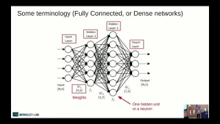
So
in
this
there
are
a
few
terminology
here
to
remember
this
is
the
input
layer
called
an
input
layer.
B
B
Each
hidden
layer
has
a
bunch
of
parameters,
these
are
weights
and
they
also
have,
and
then
there
is
an
output,
their
activations.
So
the
idea
of
activations
is
essentially
that
idea
of
having
a
non-linearity
and,
and
then
your
network
and
the
way
that
it
works,
is
that,
as
you
saw
before,
we
have
a
number
of
features,
those
number
of
features
they
are
weighted.
We
calculate
their
weighted
sum,
which
is
essentially
by
multiplying
them
by
W.
We
add
a
bias.
We
pass
that
through
an
activation
function
and
we
call
that
the
output
of
the
activation
function.
B
This
is
where
the
analogy
to
real
neurons
comes
in
the
ideas
you
have
done,
the
writes
those
dendrites,
they
collect
signal
from
different
places
and
then
the
neuron
decides
whether
to
fire
or
not.
And
then
you
have
the
output
signals
which
goes
into
other
neurons
bit
of
terminology
here.
The
number
that
we
calculate
the
weighted
sum
is
called
a
pre
activation.
The
output
of
the
activation
function
is
called
the
activation
of
that
neuron.
B
So
how
do
these
activations?
Look
like
not
the
activations
the
activation
functions,
so
there
is
a
variety
of
them
and
if
you
look
at
papers
right
now,
you'll
see
that
only
a
few
of
these
appear.
We
will
talk
about
them
in
in
details,
some
of
them
at
least
in
details.
So
if
you
look
at
most
of
the
recent
papers,
you
will
see
that
riilu
is
the
most
common.
A
rectified
linear
unit
is
the
most
common
non-linearity.
B
Essentially
it
takes
the
input
and
if
the
input
is
positive,
it
passes
it
linearly
at
the
end,
but
is
negative.
It
just
chops
that
out
we'll
see
if
this
is
a
good
idea
or
not
a
leak,
you
riilu
has
the
same
thing,
but
it
leaks.
Some
part
of
the
negative
input
and
the
exponential
linear
unit
is
is
similar
to
the
to
the
raloo
and
and
in
the
positive
regime.
So
essentially
it's
near
in
there,
and
then
it
has
an
exponential
in
the
in
the
negative
region.
B
The
reason
that
we
use
any
of
them
or
one
of
them
or
the
other
is
mainly
because
of
computational
efficiency
and
also
for
optimization
ease.
Is
it
easier
to
optimize
a
neural
network
with
one
of
these
versus
the
other?
Sometimes
you
want
to
try
in
your
own
network
and
see
that
one
of
them
works
better
for
you
they
can
the
tantor
the
hyperbolic,
hyperbolic
tangent
you
you
see
this
mostly
in
recurrent
models
nowadays,
I
think
you
will
hear
more
about
this
later
this
week.
Sigmoids
and
Contra
are
also
used
in
as
output
layers.
B
B
Hypertension
hyperbolic
goes
from
minus
1
to
1.
This
also
is
a
nice
property
that
you
might
be
looking
for.
Ok,
so
that's
a
that's!
What
a
neural
network
is
now
we
said
that
we
want
to
build
this
mirror
network
to
try
to
approximate
some
relationship
in
the
right,
but
what
sort
of
relationships
can
we
approximate?
B
There
is
a
theorem
that
appeared
in
early
90s.
It's
called
a
universal
approximation.
Theorem
theorem
says
essentially
this
that
if
you
have
a
neural
network
with
one
hidden
layer,
it
can
approximate
any
continuous
function.
That
is
there,
given
that
you
can
have
as
many
neurons
or
hidden
units
in
that
layer
as
possible,
essentially
in
their
neural
network
with
a
linear
output
unit,
can
approximate
can
approximate
any
continuous
function,
arbitrary,
well,
given
enough
hidden
units.
B
So
the
reason
that
this
is
an
important
result
is
that
we
have
a
theoretical
guarantee
that
if
we
have
the
right
architecture-
and
if
you
have
the
right
capacity,
we
will
be
able
to
approximate
that
Easterns
principle
we'll
be
able
to
approximate
the
relationship
that
we
have
in
data
now.
Of
course,
this
theorem
doesn't
mention
anything
about
how
easy
it
is
to
find
the
parameters
of
of
such
a
network
right.
B
So
you
can,
you
can
have
random
parameters,
but
you
don't
necessarily
have
a
method
finding
the
right
parameters
to
approximate
your
function,
and
it
also
doesn't
mention
anything
about
it.
Also
missa
Tate's
here
an
arbitrary
number
of
hidden
units
and
that's
not
practical
right,
so
you
might
not
have
enough
hidden
units
to
actually
represent
the
relationship
that
you
have
okay,
so
we
talked
about
neural
networks
as
essentially
function,
approximator
z--.
B
B
I'm
sure
you
have
come
across
this
trick
before
you
build
the
cost
function
right,
so
the
basic
idea
is
that
you
want,
if
you
have
a
certain
target-
and
this
is
all
of
this-
will
be
talking
in
the
supervised
learning
I
just
set
up
just
for
illustration,
because
it's
easier
to
list
right
here,
but
it's
the
same
thing
and
unsupervised
learning.
You
will
have
some
target
that
you
want
to
achieve.
So
the
basic
idea
is
that
you
have
some
function.
B
B
We
assume
that
the
last
function,
essentially,
if
it's
high,
then
it's
bad.
If
it's,
if
it's
small,
that
means
the
output
of
the
neural
network
is
very
close
to
the
real
target,
and
then
you
average
all
of
that
over
all
of
your
data
set.
We
call
that
the
cost
function,
so
the
cost
function
is
essentially
the
average
over
many
examples
of
their
real
training
data
set.
B
Okay,
there
is
a
framework
called
empirical
risk
minimization.
So
if
you're
looking
at
any
sort
of
introductory
course
and
machine
learning
or
in
deep
learning,
you
will
see
this
this
framework.
The
basic
idea
is
that
what
we
really
want
to
achieve,
we
don't
want
to
have
our
network
do
very
very
well
on
the
training
data
set,
but
we
are
really
trying
to
do
is
to
have
it
do
well
on
a
data
set
up.
It
hasn't
seen
before
right.
This
is
what
we
call
the
generalization
error.
B
We
want
it
to
actually
generalize
beyond
the
data
set,
that
we
have
the
two
concepts.
So,
if
we're
only
trying
to
make
it
work
on
the
training
data
set,
that
would
be
called
optimization
if
we're
trying
to
make
it
work
on
an
unseen
data
set.
That
would
be
called
learning
right.
That's
the
goal
of
learning,
so
the
real
goal
is,
is
to
actually
have
the
cost
function
on
the
entire
data
set
to
be
really
really
low.
The
entire
data
set.
B
This
is
the
actual
the
data
generation,
Distasio
generation
distribution,
the
original
source
of
your
data
set,
but
we
don't
have
access
to
this
one.
This
would
be
called
the
true
risk,
that's
what
we
are
trying
to
minimize,
but
what
we
end
up
minimizing.
We
end
up
minimizing
the
empirical
risk,
which
is
the
same
quantity,
but
averaged
over
the
training
data
set
that
we
have,
and
we
call
this
the
empirical
risk.
B
The
reason
that
I
wanted
to
point
this
out
is
because
this
is
generally
the
at
least
a
theoretical
framework
from
where
all
of
this
starts
we're
trying
to
minimize
the
real
risk
on
data
generation
distribution,
but
we
end
up
doing
an
optimization
over
the
training
data
set,
and
then
we
hope
that
it
will
do
well
on
an
unseen
data
set.
Okay.
This
is
a
great
principle,
but
it
doesn't
in
reality,
it's
not
very
it's
good
to
to
think
about,
but
it's
not
how
we
build
these
cost
functions.
B
For
many
reasons,
it
turns
out
that
most
of
the
of
their
losses
that
we're
interested
in
this
empirical
risk
or
the
risk
that
that
we're
interested
in
most
of
the
time
it's
not
smooth,
so
you
can
think
of
the
risk
if
you're
trying
to
classify
cats
and
dogs.
What
you're
really
trying
to
to
say
is
this
image
a
cat
or
a
dog?
So
it's
a
zero
one
sort
of
risk
you
either
it's
either
a
dog
or
a
cat.
There's
no,
like
you
don't
give
me
problems
like
the
real
risk,
is
not
probabilities.
B
B
B
B
B
B
Normally,
that's
an
assumption,
so
you
say
that
the
difference
between
y
and
the
function
and
the
output
of
your
neural
network
I
want
that
to
be
distributed
normally
or
I,
assume
that
the
real
errors
and
the
data
sets
are
distributed
normally,
and
this
is
an
a
good
assumption
right.
It
says
that
if
the
if
the
output
of
the
neural
network
is
very
close
to
the
real
output,
it's
okay,
but
if
it's
very
very
far,
I
want
you
to
penalize
strongly
right.
So.
B
If
I
have
P
model
is
a
normally
normal
distribution,
I
can
plug
that
into
the
log-likelihood
and
then
P.
Remember
the
normal
distribution
is
exponential
to
the
power
of
the
mean
minus
the
F
here,
which
is
the
x
squared
and
then,
when
you
have
the
log,
it
cancels
the
exponential
and
you
end
up
with
there
l2
loss,
and
this
is
essentially
how
you
think
of
this
is
using
the
maximum
likelihood
to
build
the
l2
loss
in
a
similar
fashion.
B
B
Gradient
descent
right
like
this
is
the
oldest
trick
in
the
book.
You
have
a
function
you're
trying
to
minimize
that
function.
How
do
you
do
that?
You
take
the
derivative
at
the
point
where
you
are
and
then
the
derivative
points
in
the
direction
where
the
function
is
increasing
negative,
that
that
will
be
the
descent
direction,
and
then
you
take
one
step
in
the
direction
of
your
descent
and
you
update
your
parameters
all
right.
So
mathematically,
you
have
your
WK
and
then
you
take
the
gradient.
B
Okay.
You
need
to
remember
that
we're
talking
about
the
learning
great
or
the
step
size
where
this
is
where
it
comes
in.
We
will
talk
a
bit
about
this
later.
In
reality,
this
gradient
gradient
descent.
When
we're
talking
about
just
gradient
descent,
we
mean
take
your
entire
training
data,
set,
evaluate
the
gradient
on
the
entire
training
data
set
and
then
make
one
step
this
is
it
doesn't
work
really
in
reality
right.
Your
dataset
can
be
millions
of
images,
it's
extremely
expensive
to
actually
evaluate
your
last
function
on
the
entire
data
set.
B
Another
thing
is
that
you
don't
want
your
training,
the
complexity
of
your
of
training
or
optimizing.
Your
network
to
grow,
as
your
data
set,
is
growing
right
if
I
am,
if
I'm,
essentially
increasing
that
I'm
evaluating
the
entire
gradient
on
the
entire
data
set.
That
will
be
all
n
complexities,
linear
complexity,
but
you
don't
want
that.
So
in
practice
we
use
the
gradient
that
stochastic
gradient
descent.
B
We
say
instead
of
using
the
full
gradient,
let's
evaluate
the
gradient
approximate
that
or
with
just
a
small
number
of
of
examples
from
the
dataset,
and
we
hope
that
that
is
you
know
it's
good
enough.
It
will
give
me
a
good
idea
of
which
direction
to
go,
but
the
one
I
rely
too
much
on
on
the
gradient.
This
is
what
we
call
stochastic
gradient.
Descent
is
stochastic
because
those
examples
are
presumably
random,
so
you're
picking
them
randomly.
B
You
don't
want
to
have
a
lot
of
correlations
in
the
in
the
randomness
of
your
gradient,
so
this
came
in
the
beginning.
It
came
out
as
an
idea
for
how
to
do
this
iterative
process
of
doing
gradient
descent
or
optimization
much
faster
in
practice.
What
we
realized
is
that
the
noise
that
you
get
from
the
stochastic
nature
of
this
gradient
estimate,
essentially
the
difference
between
this
gradient
value
from
small
small
number
of
examples
and
the
full
data
set.
It
turned
out
that
that
noise
in
itself
is
extremely
important
to
optimize
these
neural
networks.
B
We
will
see
and
we'll
see,
a
plot
later
of
how
the
last
function,
the
surface
of
this
last
function,
might
look
like,
so
essentially
that
noise,
at
least
intuitively.
It
helps
to
kick
your
network
or
your
parameters
out
of
local
minimums,
so
that
it
goes
to
a
more
a
global
minima
and
in
fact
it
turns
out
that
the
larger
the
batch
that
we
use
the
more
problems
we
have
in
finding
there
are
a
good
many
minimizer
of
the
entire
network.
B
So
you
will
see
I
think
during
this
week
you
will
see
a
lot
of
discussions
of
large
batch
training.
How
do
I
do
training
with
a
larger
batch
okay,
so
two
things
to
point
out
here
is
that
the
learning
rate
and
the
mini
batch
size.
How
many
examples
do
you
want
to
use
in
every
step?
These
are
hyper
parameters,
and
these
are
examples
of
two
hyper
parameters
that
are
extremely
important
to
find
good
parameters
to
train
your
network
and
then
we'll
talk
more
about
this.
B
In
my
talk
and
then
also
in
other
talks,
there
is
a
hpo
talk
later
in
the
week.
Hyper
parameter,
optimization
talk
that
discusses
just
how
to
do
this.
This
stuff,
generally
right
now
to
first-order
using
a
small
batch
somewhere
between
1
and
32
and
powers
of
2,
is
reasonable.
This
is
what
you
will
see
in
most
in
practice.
Once
we
have
once
the
community
has
experience
with
a
certain
network,
you
start
seeing
larger
and
larger
batch
sizes,
for
example
ResNet.
You
will
see
that
most
of
the
time
people
train
with
256
batch
size.
Yes,.
B
B
Actually
there
is
a
lot
of
research
recently
that
is
doing
just
that,
but
so
essentially
it
says
that
when
I
am
when
I
start
from
random
parameters
at
the
very
early
stage,
I
want
to
have
as
much
noise
in
my
gradient
as
possible,
and
then
I
use
a
small
batch
size
to
make
my
steps
I'm
still
exploring
trying
to
kick
myself
out
of
all
the
local
mini
months,
but
once
I
get
to
a
flat
region
and
the
last
surface
I
can
take
a
more
confident.
There
are
less
problems.
B
B
Okay.
So
how
does
this
look
in
practice?
I
just
want
to
emphasize
that
yeah.
When
you
use
learning
great
that
are
off,
you
will
get
differently
lost,
curves
or
learning
curves,
and
you
will
need
to
really
need
to
find
the
right
learning
rate
okay.
So
how
do
we
find
the
the?
How
do
we
actually
do
this
in
practice?
So
if
you,
if
you
look
at,
if
you
look
at
examples
trying
to
visualize,
there
are
a
lot
of
these
we're
trying
to
visualize
the
last
surface
of
a
real
neural
network
on
a
real
data
set.
B
You
will
see
examples
like
this.
So
I
think
this
is
for
vgg
56,
which
is
one
of
the
winners
of
the
imagenet
competition
standard
model.
People
have
done
a
lot
of
stuff
with
it,
and
this
is
a
visualization
of
the
lost
surface
at
a
certain
point,
during
the
training
the
way
that
they
do
this,
they
try
to
find
two
directions
in
which
the
last
changes
the
most
and
then
try
to
visualize
it,
because
you
know
these
networks
have
tens.
B
If
not
hundreds
of
millions
of
parameters,
you
want
to
choose
two
directions
to
visualize,
to
make
a
surface
like
this.
Unfortunately,
we
can
plot
in
more
than
more
dimensions.
So-
and
you
get
something
like
this,
you
can
immediately
see
that
sort
of
trouble
that
you
can
run
into
right.
You
can
get
stuck
in
a
lot
of
local
minimis
if
you're,
if
you're
learning
great,
doesn't
doesn't
essentially
kick
you
out
of
these
local
minimums.
If
you
don't
have
enough
noise,
you
will
not
get
to
a
location
like
this
right.
B
You
can
also
see
that
you
can
get
stuck
optimizing
like
and
in
certain
places
you
can
get
stuck
in
saddle
points
right
instead,
just
like
you
know
in
your
in
your
pace,
you
can
also
see
immediately
here
that,
if,
if
you're,
for
example,
your
parameters
are
somewhere
on
the
surface
and
then
you're
you're
lost
you're,
your
learning
rate
is
very
small.
You
won't
travel
far
from
where
you
have
started
right,
but
if
your
learning
rate,
it
is
very
large,
it
can
essentially
catapult
you
all
the
way
to
arrive
in
somewhere
far
away.
B
B
There
is
a
range
of
optimizers
people,
don't
use
just
gradient
descent
in
practice.
The
first
thing
that
you
can
think
of
is
that
you
can
have
a
momentum
right.
So
if
you
have
a
ball
rolling
down
surface,
you
can,
instead
of
trying
to
do
only
locally
trying
to
make
your
step
based
on
the
local
gradient.
You
can
accumulate
your
speed
right
while
you're
coming
down
and
then
use
that
to
kind
of
give
you
a
sense
for
where
you
should
go.
The
general
direction
right,
so
stochastic,
gradient,
set
with
momentum,
would
be.
B
The
very
first
thing
to
do.
Nesterov
is
a
variation
over
this,
which
is
essentially
UI.
First
update
my
location
based
on
my
velocity
and
then
evaluate
the
gradient
or
or
evaluate
the
gradient
update,
and
there
is
a
range
of
other
things
like
other
grad
and
rmsprop.
Essentially,
they
try
to
use
the
size
of
the
of
the
gradient
along
the
way
to
estimate
by
the
size
of
the
step
that
you're
taking
once
you
get
into
other
grad
and
rmsprop.
We
start
having
different
learning
rates
for
different
crimes.
B
Different
updates
scales
for
different
parameters-
and
then
you
have
Adam
Adam,
is-
is
essentially
doing
somewhat
of
Armas
prop
Plus
momentum,
so
it
combines
the
two
ideas
and
then
it
also
tries
to
eliminate
any
bias
in
the
estimates
of
the
estimates
of
the
the
gradient
mean
and
and
variance.
This
is
very
high-level,
I'm
gonna,
probably
if
we
have
time
we
can
get
into
the
details
of
these
different
optimizers
tomorrow,
you
can
see
in
a
plot
like
this,
that
some
optimizers,
for
example,
pure
as
GD,
gets
stuck
there.
B
Of
course,
this
is
kind
of
a
diagram
just
to
show
in
principle
how
this
happens.
If
the
learning
rate
is
different,
it
might
not
get
stuck
right
if
there
is
some
noise
and
the
gradient,
it
also
might
not
get
stuck.
But
this
is
just
to
illustrate
the
idea
right
and
you
can
see
that
other
sort
of
optimizers.
B
B
That's
true,
so,
in
practice,
what
we
have
realized
is
that
a
lot
of
these
optical
parameters,
these
optimizers,
they
make
it
easy
to
optimize
network.
If
you
don't
know
what
parameters
to
use
so,
but
in
practice
the
best
sort
of
generalization
error
comes
when
you
use
as
gd+
momentum,
but
it
takes
a
lot
of
hyper
parameter,
optimization
to
be
able
to
find
the
right
parameters.
B
So
I
think
this
is
also
something
that
Brenda
I
mentioned.
Is
that
when
you
use
something
like
Adam,
you
don't
worry
a
lot
about
the
exact
value
of
your
learning
rate,
but
the
best
value.
At
least
you
can
start
experimenting
with
the
rest
of
your
model
without
having
to
worry
so
much
about
this
being
completely
off.
It's
less
sensitive
to
the
exact
value
of
the
learning
rate.
But
if
you
look
at
most
of
the
the
state-of-the-art
results
like
models
like
resonate,
for
example,
you
see
that
they
actually
use
SVD
plus
Compton.
B
B
The
other
question,
okay,
so
I
said
we
have
a
loss
function.
We
take
the
gradient
of
that
loss,
function
with
a
certain
parameter
and
then
the
parameter
of
the
network,
and
then
we
take
one
step
opposite
to
the
gradient
right.
But
we
have
a
lot
of
parameters
in
these
networks.
How
do
we
get
the
parameters
to?
How
do
we
get
to
the
parameters
inside
the
network
themselves?
Not
at
the
very
last
layer
and
the
output
layer?
B
For
example,
we
use
again
the
oldest
trick
in
the
book,
which
is
the
chain
rule
of
calculus
to
propagate
the
errors
from
the
last
function,
all
the
way
to
the
parameters
that
were
trying
to
update.
So
imagine
this
is
the
output,
Z
and
you're
trying
to
get
you're
trying
to
update
W.
You
need
to
actually
pass
through
the
entire
network.
Partial
C
by
partial
W
would
be
partial,
X,
partial
W,
partial
Y,
partial
X,
partial
Z,
but
partial
Y.
B
This
is,
if
you're
taking
a
class
like
CS
231.
You
will
see
that
they
spend
at
least
a
whole
lecture
an
hour,
15
minutes
talking
only
about
back
propagation,
how
you
do
actually
this
in
practice,
there
are
a
lot
of
things
that
you
want
to
to
take
care
of.
Essentially
how
do
you
do
it
efficiently
on
linear
ax,
on
on
modern
ax
aerators,
but
for
the
conceptual
understanding
of
how
things
work?
B
All
you
need
to
remember
is
that
there
is
a
chain
rule
and
your
gradients
are
actually
propagating
to
all
the
other
factors
that
you
have
in
your
network,
and
this
is
very
important
because
imagine
that
one
of
these
is
zero.
Imagine
that,
like
one
of
these
is
zero
or
one
of
them
is
extremely
small.
You
will
not
have
any
gradient
signal
going
back
to
area
layers
right,
which
would
kill
the
update
to
2
W
immediately
can
also
think
of.
If
this
is
extremely
large,
it
will
also
support
the
whole
thing
off.
B
B
Is
the
most
common
now
activation
function
and
the
networks
that
you
see
around
and
the
basic
form
of
the
function?
If
it's
linear
the
input
is
linear.
If
the
input
is
positive,
you
go
to
a
linear
response.
If
the
input
is
negative
at
zero,
there
are
a
lot
of
good
properties
about
this.
First
of
all,
it's
computationally
cheap.
It's
extremely
cheap
right.
B
The
other
and
compare
this
to
the
sigmoid
that
has
an
exponential,
we'll
talk
about
this
in
a
bit
it
has
exponential,
are
very
expensive
to
calculate.
Initially,
people
thought
that
sigmoid
would
be
a
good
way
to
do
it.
The
other
thing
is
that,
when
it's
positive,
the
slope
of
this
function
does
not
alter
the
the
slope
of
the
actual
output
of
the
neuron.
It
can
give
very
strong
gradient
signals
right.
B
You
see,
it's
not
dying
like
other
functions
right,
so
if
the
slope
here
is
good
to
for
a
gradient
propagation,
one
of
the
issues
with
riilu
is
that
if
the
output
is
negative
of
your
neurons
negative
it
essentially,
it
kills.
The
EO
kills
the
output,
but
also
kills
the
gradient
right.
We
just
said
that
if
this
has
slope
0,
so
there's
nothing
will
propagate
back,
so
this
leads
to
dead
neurons.
B
B
So
one
way
to
get
around
this
is
to
use
something
called
leaky
riilu,
which
is
essentially
keep
some.
You
use
some
some
part
of
the
negative
negative
part
of
the
of
your
input,
so
you
have
Alpha
X
alpha
times.
X
X
would
be
negative
here
right
and
then
alpha
between
0
&
1,
which
is
essentially
you
keep
some
leakage
in
your
function
so
that
gradients
can
propagate
back,
and
this
is
this
is
very.
This
is
very
important
in
practice.
B
You
will
see
that
one
of
the
ways
to
actually
monitor
if
your
network
is
doing
well
or
not,
is
to
look
a
lot
on
how
many
neurons
are
not
dead.
Okay,
two
other
activations
I
want
to
talk
about
the
first
one
is
sigmoid
so
sigmoid.
We
don't
use
it
inside
the
neural
networks
in
the
head
and
after
hidden
layers,
so
inside
the
neural
networks
anymore,
you
might
find
it
that's
it.
You
might
find
a
lot
of
things,
but
in
practice
we
use
it
to
represent
probabilities.
B
So
if
the
output
of
my
neural
network
has
to
be
somewhere
between
zero
and
one,
it's
very
easy
to
just
take
the
output
of
the
neural
network.
It
should
be
on
the
x-axis
and
then
that
will
give
me
it
will
squash
that
x-axis
into
0
to
1-
and
this
is
great
right
for
representing
Bernoulli
distribution-
it's
expensive
to
you
to
compute.
However,
if
you're
only
using
it
at
the
very
last
layer.
It's
ok
right.
B
One
thing
that
I
want
to
mention
about
sigmoid.
Is
that
actually
they
only
say
so
a
lot
of
what
you
will
see
right
now
and
stuff
that
you
think?
Oh,
this
is
great,
and
this
is
what
happens
to
all
of
us.
You
understand
the
different
details,
but
after
you
get
into
deep
learning
in
practice,
especially
if
you
are
in
application,
applying
deep
yearning
for
science,
not
doing
deep
learning
research,
you
get
into
the
practice
of
doing
neural
networks
as
plug
and
play.
So
you
say:
oh,
this
is
I.
B
Want
this
output
I'm
gonna
try
with
the
output,
which
is
between
0
and
1,
and
that
is
a
sigmoid
function,
gives
me
0
1,
that's
very
nice
and
then
you're
gonna
say:
oh
I'm
gonna
try
different
classes,
I'm
gonna,
try
maximum
likelihood,
I'm
gonna,
try,
l1
I'm
gonna,
try
l2,
and
there
are
fundamental
reasons
for
why
that's
a
bad
idea
to
use
any
random
loss
with
any
round
activation
function.
One
of
them
is
this
one,
so
you
can
see
here
that
the
output
of
a
sigmoid
it
has
extremely
vanishing
like
this
is.
B
B
B
B
B
Yes,
I
see
your
question,
so
the
question
is
release.
They
seem
to
be
linear
because
they
always
output
everything
linearly
right,
except
when
it's
positive,
when
it's
negative
and
the
answer
and
how
come
this
is
a
nonlinear
function,
the
answer
it
is
nonlinear,
because
the
fact
that
you're
actually
killing
the
negative
part
produces
all
of
these
farce
representations
when
you
compose
a
lot
of
them
after
each
other
you're
creating
you
know,
nonlinear
big
nonlinear
functions
and
the
idea
of
riilu
by
the
ways
it's
also
connected
or
inspired
by
nuance.
B
You
have
done
the
writes
and
then
they
either
respond
or
they
don't
respond
some
time
the
whole
neuron
might
respond
or
not.
And
then,
if
it's
just
a
zero
one
sort
of
response
you
still
create,
you
can
create
nonlinear
functions.
Okay,
so
the
point
I
was
trying
to
make
here
if
you're,
using
a
sigmoid.
Remember
that
you
have
an
exponential
in
there.
You
remember
that
you
have
this
vanishing
gradient
and
then
remember
that
that
needs
a
log
to
undo
the
exponential.
B
B
B
So,
in
this
case,
like
Bernoulli,
we
are
assuming
that
the
data
is
the
the
actual
output
is
distributed
according
to
her
knowledge
distribution,
we're
trying
to
match
that
it's
it's
much
better
for
learning,
it's
easier
to
actually
optimize
networks
with
these
distributions,
rather
than
to
try
to
optimize
on
the
original
distribution
that
it's
like
0
1,
for
example,
that
we're
looking
for
I.
Think
it's
it's
easier
to
illustrate
this
with
the
softmax,
because
you
have
a
you,
have
a
so
the
question.
So
ok,
so
we
talked
about
the
sigmoid.
B
It's
great
to
to
represent
binary
sort
of
probability
is
some
number
between
0
and
1,
and
the
question
is
whether
why
is
this?
What
if
this
doesn't
actually
represent
the
data
set
right
in
your
data?
You
have
it's
either
a
dog
or
a
cat.
It
doesn't
have
probabilities
in
between
and
trying
to
say
that
we,
this
idea,
is
connected
to
the
idea
that
we're
using
surrogates
loss
functions
because
they
are
easier
to
actually
handle
in
the
optimization
process.
B
Now,
if
what,
if
we
have
multiple
categories,
not
daksa
cats
and
dogs,
but
we
have
ten
ten
different
categories.
What
do
we
do?
So
we
again
assume
that
there
is
something
the
data
has
some
distribution.
In
this
case.
We
assume
that
there
is
a
multi,
only
output
distribution,
and
this
will
be
multi
class
out,
but
in
reality
the
real
rest
things
like
this,
for
example,
if
you're
looking
at
colors
the
colors
are
color,
is
not
the
best
to
explain
this,
but
categories
of
animals.
B
Your
categories
are
really
like:
it's
either
this
animal
or
that
it's
not
probabilities
over
those.
However,
using
this
idea
that
we
have
a
distribution
over
all
possibilities
makes
it
easier
to
actually
optimize
the
neural
network.
So,
when
you're
looking
at
an
MS
trying
to
identify
the
animal
in
that
image,
you
assume
that
there
is
a
multinomial
distribution
and
they
have
different
probabilities
of
being
different
animals,
and
that
is
not
reading
the
distribution.
B
Does
that
kind
of
answer
your
question?
We
can
talk
about
it
later:
okay,
so
multi,
no
lis
distribution.
The
idea
is,
how
do
I,
if
I,
have
a
multi-class
problem?
What
sort
of
loss
function
do
I
use?
What
sort
of
how
do
I
guarantee
that
the
output
of
my
network
can
actually
give
me
something
that
tells
me
which,
to
which
class
does
the
object?
Does
the
input
belong
and
the
idea
is
to
use
the
softmax
function?
B
The
softmax
function
says
essentially
exponentiate
all
of
your
the
output
of
all
the
layers,
so
all
of
these
layers
exponentially
at
their
output
and
then
normalize
them
by
the
total
right,
so
that
and
that
would
be
the
output
for
every
category,
and
this
is
essentially
gives
you.
The
sum
of
this
over
all
categories
would
be
one
because
that's
the
denominator
right
and
then
the
value
of
each
one
of
these
would
be
the
probability
that
the
input
belongs
to
any
of
the
objects
that
you
have,
so
it
does
produce
a
distribution
of
our
classes.
B
This
is
different
from
trying
to
tell
if
two
different
objects
are
within
the
within
an
image
or
not
like,
for
example,
if
there
is
a
probability
that
there
is
a
dog
and
there
is
a
cat.
In
that
case,
you
want
to
use
a
soft
max.
You'd
use
a
sigmoid
over
two
different
neuron
outputs,
okay.
So
the
way
that
you,
you
use
the
information
that
comes
out.
You
say
that
the
class
with
the
largest
probability,
that
would
be
the
class
of
the
object.
So
that
would
be
the
guess
of
the
network.
B
The
if,
if
the
data
is
noisy,
that
your
labels
themselves
would
be
noisy,
so
the
neural
network
would
try
to
do
whatever
is
the
target
that
you
have
in
your
own
data
set?
If
and
that's
a
question
like
that,
comes
back
to
you
that
can
you
tolerate
that
noise
in
your
data
set
or
not,
and
if
you
can
tolerate
it,
how
do
you
want
to
handle
it?
If
not,
you
want
to
remove
it,
and
this
goes
back
to
yeah.
So
I
think.
Does
that
answer
your
question?
B
Instead
of
using
regression,
we
classify
our
output,
we
know
that
the
output
has
to
have
a
range
between
minus
ten
and
ten.
We
divide
that
into
different
categories,
and
we
try
to
use
a
soft
max
to
predict
a
distribution
over
over
these
different
bins,
rather
than
try
to
predict
a
particular
number,
and
this
is
for
many
reasons.
B
The
other
thing
is
that
the
when
you're
using
you're
doing
regression
and
the
output
of
your
neural
network
is
linear,
you're,
really
trying
to
you're
asking
the
network
to
output
that
particular
number,
but
when
you're,
when
your
output
is
exponentiate
like
this
all
you're
asking
the
neural
network
is
to
guess
some
good
number
right,
because
because
the
number
really,
if
it's,
if
it's
maybe
three
or
ten,
it
will
probably
give
me
the
same
category.
It
will
give
me
that
in
the
same
range,
so
the
neural
network
has
much
bigger
range
to
play
with
to
output.
B
B
So
if,
if
your
data
is
wrong,
if
it's,
if
your
label
says
it's
green
and
it's
not
green,
then
it
will
just
memorize
that
and
your
learning
will
be
bad.
It's
you're
not
going
to
learn
something
that
generalizes
well,
if
you
have,
if
you,
if
the
data
is
just
noisy,
there's
a
distribution
over.
Maybe
this
is
like
you're
showing
a
certain
color.
B
B
These
are
two
cases
but
I'm
sure
there
are
so
many
other
cases
in
between
that.
You
need
to
handle
them
one
by
one.
Okay,
so
I
want
to
get
into
I.
Think
I
have
20
minutes.
Okay
have
20
minutes
ago,
so
I'll
get
into
a
few
topics
that
are
important
before
we
carry
on
with
the
rest
of
the
day.
First
of
all,
Brenda
talked
about.
B
How
do
you
monitor
your
neural
networks,
learning
and
I'm
sure
this
idea
that
you
have
also
seen
it
before
right
again,
what
we're
trying
to
do
we're
not
trying
to
optimize
we're
trying
to
learn
so
we're
trying
to
generalize
beyond
the
data
set
that
we
have.
So
if
you
look
at
the
error
of
your
front
viewer,
your
neural
network
output
or
the
last
function
or
any
surrogate
for
this
quantity,
and
then
you
evaluate
that
on
your
training
data
set,
it
should
be
going
down
all
the
time.
B
So
optimization
has
happened
right,
however,
we're
trying
to
generalize
to
some
other
data
set.
So
we
usually
split
the
original
data
into
three
categories:
a
training
data,
a
validation
data
and
a
test
data
set.
The
test
data
set.
You
just
hide
until
the
very
last
day
before
you
submit
your
papers,
so
very
last
night,
don't
even
bother
trying
to
do
anything
on
the
test
data
set.
This
is
extremely
precious.
You
really
don't
want
to
do
it.
B
You
don't
want
to
look
at
it
at
all
until
the
very
last
minute,
the
validation
data
set
I
prefer
a
different
name
for
it's
called
the
development
data
set.
Sometimes
you
even
spread
that
validation
into
two
data
sets.
One
of
them
is
called
development.
The
other
one
is
validation.
The
development
data
set
is
something
that
you
use
to
tune
your
hyper
parameters.
The
the
validation
data
set
is
to
monitor
the
learning
process
tuning
the
hyper
parameters.
You
don't
want
to
over
tune
them
to.
B
Actually
you
know
your
overfitting
to
the
actual
validation
data
set
that
you
have
that's.
Why?
Sometimes
you
you
keep
a
development
data
set
aside.
The
breakdown
of
this,
the
general
consensus
is
80/10/10.
You
will
see
a
lot
of
60
20,
20
or
any
other
variation
I
prefer
to
have
as
large
of
validation
and
test
data
sets
as
possible,
because
you
really
don't
want
to
fool
yourself
right.
Like
you
don't
want
to
come
out,
oh
it's
great
you're.
B
If
you're
really
trying
to
do
science,
we
want
to
have
confidence
that
you're
really
doing
the
right
thing
or
your
network
is
doing
the
right
thing
now.
How
do
these
these
curves
look
like?
There
are
multiple
regimes:
if
you're,
comparing
to
the
training
data
set
to
you,
there
is
the
and
the
validation
there's
the
regime
where
you're,
essentially
your
model
is
underfitting.
Underfitting
means
that
you're
not
even
doing
well
on
the
training
data
set
itself,
and
that
has
there
are
many
things
that
you
need
to
check.
B
We
will
get
into
some
of
these
tomorrow,
but
the
very
first
thing
you
are:
you
want
to
see
if
you
have
a
bug
in
your
net
in
your
code
before
any
of
these,
if
you're
underfitting
after
that,
you
want
to
probably
check
your
model
architecture
and
stuff.
Actually
before
that,
you,
you
want
to
check
your
learning
rates
before
the
model
architecture,
because,
if
your
learning
rate
imagine
if
it's
extremely
small,
that
means
you're
not
really
getting
you're,
not
taking
large
steps.
B
You
know
that
are
large
enough
to
get
to
a
minimum
and
it
just
gonna
take
forever
to
get
to
to
a
meaningful
minimum.
So
you
wanna
check
the
learning
rate
after
that
you
probably
want
to
look
at
the
model
architecture.
If
this
check
out,
you
probably
want
to
either
train
longer
or
look
at
either
other
hyper
parameters.
These
are
of
no
particular
order
at
the
moment,
but
tricking
the
learning
rate
would
be
the
very
first
thing.
I
want
to
emphasize
that
the
validation
error
and
the
training
error
being
close
to
each
other.
B
All
the
time
is
that
you
are
underfitting,
so
even
if
your
you
have
trained
for
three
days
and
they
are
still
extremely
close
to
each
other,
you're
still
underfitting
very
likely
you're
still
underfitting,
you
need
to
check
what's
going
on
especially
check
the
learning
rate.
The
idea
is
that
if
I
am
NOT
underfitting,
if
I'm,
not
under
fitting
the
training
glass
should
be,
I
should
be
do
much
better
on
my
training
data
set
than
on
my
validation
visa,
because
these
neural
networks
they're
over
optimum
parametrized,
they
are
extremely
powerful.
B
B
So
the
overfitting
regime
I
do
very
well
on
my
training
data
set
and
not
that
well
on
the
validation
that
kind
of
comes
down
and
then
start
climbing
as
soon
as
starts
climbing
I
know
that
I
started
overfitting.
This
is
what
we
call
the
generalization
gap,
and
this
is
what
you
spend
most
of
your
time,
trying
to
close
this
generalization
gap,
we're
trying
to
move
essentially
this
point
to
much
further
along.
B
B
Some
of
them
is
essentially
the
learning
rate
where
there
could
be
problems
with
the
learning
rate.
The
data
set
could
be
not
enough
right.
If
you
don't
have
enough
data
set,
you'll
probably
want
to
increase
that
there
are
ways
if
you
can't
go
and
collect
more
data.
There
are
ways
to
augment
the
data
set
that
you
have.
You
can
do
that
and
then,
once
all
of
these
things
check
out
you're
welcome
to
deep
learning,
you
start
doing
regularization.
So
regularization
techniques
are
the
stuff
that
we
will
talk
about
tomorrow.
B
If
your
it
depends
on
the
problem,
really
it
could
be
that
your
model
is
not
learning
really
as
fast
enough,
so
you
probably
have
connections
that
have
problems
on
them.
You
have
bottleneck
layers
that
are
too
narrow
for
your
model
to
learn,
but
in
the
general
sense,
yes,
you
want
to
check
the
number
of
layers
that
you
have
the
sizes
of
each
of
the
layers
and
all
of
that,
if
you're
not
overfitting
to
the
training
data
set,
there
is
something
terribly
wrong.
We'll
talk
about
this
under
fitting.
B
A
B
Point
this
is
what
we
call
the
early
stopping
point,
which
is.
Essentially
you
want
to
stop
the
training
as
soon
as
your
validation
error
starts
climbing
and
it's
a
sort
of
a
regularization
technique.
We'll
talk
about
this
okay,
so
I
have
15
more
minutes
and
I
want
to
get
into
the
last
topic
for
today,
which
is
convolutional
neural
networks.
B
So
you
can
build
all
of
all
sorts
of
functions,
so
we
saw
a
set
up
where
we
have
these
fully
connected,
dense
layer
functions,
they
take
the
entire
input
and
then
try
to
give
an
output.
We
have
a
lot
of
them
stacked
after
each
other.
We
talked
about
the
universal
approximation
theorem.
We
said
that
this
particular
function
can
approximate.
If,
given
enough
capacity,
it
can
approximate
any
continuous
function
that
there
is.
B
However,
this
far
that
particular
set
up
with
the
dense
layers
doesn't
assume
and
think
about
our
dataset
right,
but
our
dates
that
we
know
that
there
are
certain
things
and
that
data
said
that
we
know
that
they're.
Absolutely
true.
For
example,
if
I
have,
if
I
have
objects
in
my
data
set,
I
know
if
those
objects
are
in
the
upper
left,
right,
upper
left
or
upper
right
or
anywhere
they
appear
in
the
data
set,
they
should
be
the
same
same
cat,
for
example
right.
B
These
sort
of
information
or
knowledge
about
the
data
set.
This
is
what
we
call
a
prior
knowledge
and
then
a
lot
of
the
work
that
goes
into
building
neural
networks
into
how
do
I
incorporate
those
prior
knowledge
or
these
constraints
or
knowledge
about
the
data
set
in
the
actual
architecture.
That
saves
me
a
lot
of
things.
First
of
all,
I'm
not
trying
to
solve
an
extremely
general
problem.
B
I'm
not
trying
to
you
know
you
know,
kill
a
fly
with
a
camera,
a
Canon
or
something
right
like
I'm,
actually
using
the
right
tool
for
the
right
job,
and
this
is
not
only
for
we'll
talk
about.
How
is
this
is
achieved
in
currency
announce,
but
this
is
in
in
science
is
actually
more
its.
We
see
that
more
often
than
in
other
other
areas.
You
can
imagine,
for
example,
Sciences
background
or
in
physics
we
always
talk
about
rotation
groups
right.
You
know
that
all
of
our
objects
are
rotationally
invariant
the
molecule.
B
However,
it
looks
like
butter
their
protein
structure.
However,
it
looks
like
it
should
stay,
it's
the
same
object
or
the
same
protein
right.
So
how
do
you
build
a
neural
network
that
respects
all
of
that?
Those
in
variances
when
we
incorporate
those
in
variances
as
infinite
priors
in
the
architecture
that
we
have?
We
tend
to
learn
first,
essentially,
models
that
general
lines
much
better
they're,
not
going
to
respect
that
on
your
training
data
set
and
then
disrespect
or
violated
on
the
validation
data
set.
B
Okay,
so
all
of
that
intro
set.
We
will
see
how
cnn's
achieve
essentially
that,
so
this
is
fully
connected
networks
that
we
talked
about
earlier
today.
You
have
your
input
is
in
blue
and
every
neuron
is
connected
to
every
single
one
of
these
inputs,
and
that's
why
we
call
it
a
fully
connected
Network.
B
One
thing
that
we
we
can
do
is
look
at.
We
do
sparse
connectivity
right
if
I
am
looking
only
if
I
am
thinking
that
only
the
local
sort
of
information
is
important
and
I
don't
have
to
correlate
pixels
or
inputs
features
that
are
far
away
from
each
other.
I
can,
just
you
know,
have
a
local
connectivity.
I
can
have
more
neurons
each
one
of
those
neurons
is
only
locally
connected
to
a
few
input
features.
I
can
do
something
further
than
that.
B
If
I
know
that
the
stuff
that
I'm
looking
for
are
the
same
wherever
they
are,
it
doesn't
really
matter
where
they
are.
In
the
end,
the
input
I
can
share
or
I
can
reuse
the
same
parameters
for
all
the
detectors
right
instead
of
having
different
parameters
here,
I
can
have
the
same
parameters
everywhere,
and
this
is
what
we
call
parameter
sharing.
So
what
does
this
bias
essentially
bias?
The
idea
of
translation
invariance
right
now,
I
have
a
instead
of
having
something
that
takes
the
entire
input
and
tries
to
output
the
gigantic
output.
B
I
have
a
much
smaller
kernel
or
small
parameters
or
a
small
detector
that
is
sliding
over
the
input
and
trying
to
produce
and
tell
me
in
this
patch
what
response
should
I
have
to
dispassion
this
patch
on
this
patch
and
I.
Do
a
lot
of
parameter,
saving
right,
any
less
parameters,
and
this
is
the
idea
of
convolutions
desire,
communes
work.
B
Essentially,
you
have
a
bunch
of
parameters,
you
slide
over
your
input
and
then
you
do
a
dot
product
with
of
your
weights,
with
your
input
right
the
bias,
and
then
you
move
on
to
the
next
two.
You
slide
the
kernel
over
and
you
move
on
to
the
next
thing
again.
What
does
this
achieve?
We
have
sparse
connectivity,
it's
only
local
responses.
We
have
parameter
sharing.
We
have
way
less
number
of
parameters,
we'll
see
an
example
in
a
bit,
and
we
also
have
translation
in
covariance.
B
You
can
check
what
the
difference,
equivalence
and
in
variances
later,
but
generally,
the
basic
idea
is:
if
I
have
an
object
in
mind.
In
my
input
it
doesn't
matter
where
that
object
is
I,
don't
need
to
learn
different
parameters
in
different
places.
This
is
again,
this
is
an
infinite
prior
on
what
sort
of
data
that
I
am
looking
at
I'm,
saying
that
my
data
has
that
property
of
being
having
objects
being
translationally
invariant
few
terminologies.
B
This
is
my
input
matrix.
We
call
it
an
input
matrix.
This
is
a
convolution
kernel
or
filter,
so
you
will
see
that
people
if
they
say
a
kernel,
that
means
it's
just
a
bunch
of
weights
that
you
multiply
by
the
input
they
can.
It's
also
called
a
filter,
so
you'll
see
that
everywhere
and
then
the
output
is
most
of
the
time
people
say
a
feature
map.
Sometimes
people
say
it's
an
activation
map,
an
example
of
how
this
works.
In
reality,
you
have
an
image.
The
image
is
52
by
32
by
3.
B
The
3
is
the
number
of
channels,
red,
green,
blue,
and
then
you
have
a
filter.
The
filter
tries,
for
example,
a
filter
5
by
5
by
3,
and
this
slides
over
the
input.
The
your
filter
has
to
have
the
same
number
like
3
to
match
the
channels
right.
So
essentially,
you
will
have
3
sets
of
5
by
5
the
parameters
to
process
your
input
and
then,
if
you
do
the
math
you'll,
you
will
see
that
your
output
is
28
by
28
activation
map
and
it
has
one
channel
here.
B
You
can
immediately
see
with
these
numbers
that,
if
I
have
just
to
ingest
this
input,
if
I
was
using
a
fully
connected
network
that
will
have
at
least
32
by
32
by
3,
that's
like
3000
or
something
and
this
and
then
multiplied
by
the
number
of
outputs
that
I
want
to
have,
but
at
least
for
one
neuron
that
would
be
about
3000
parameters
and
when
I'm
using
a
convolutional
kernel.
This
is
5
by
5
by
3.
This
is
75
parameters.
There
is
almost
two
orders
of
magnitude
reduction
in
the
number
of
parameters.
B
B
So
that's.
These
are
the
general
basics
things
about
convolutions
that
you
need
to
know.
If
you
look
at
convolutional
neural
networks,
you
will
see
that
there
is
another
type
of
layers
that
we
use.
The
essential
idea
is
that
I
have
a
lot
of
these
activations
are
coming
out
as
I
am
coming
and
coming
down
the
the
pipeline
of
convolutions.
B
Sometimes
we
want
to
to
to
reduce
the
size
of
these
feature
maps
that
are
coming
out
and
it's
interested
to
okay,
you
have,
you
are
outputting
28
by
28,
but
I
want
you
to
summarize
that
into
14
by
14.
So
and
to
do
this,
we
use
what
it's,
what
we
call
pooling
layers
so
essentially
the
pooling
layers
they
replace.
This
is
an
example
of
a
pooling
layer
with
a
kernel
size
two.
B
So
essentially
you
look
at
the
this
is
I'm
looking
at
2
by
2,
matrix
and
I'm,
then
I'm
deciding
how
to
summarize
this
2
by
2
matrix
to
another
2
by
2,
matrix
I'm,
trying
to
summarize
that
I
can
do
average
pooling
whether
I
would
average
all
of
these
numbers,
and
one
number
I
can
also
do
max
pooling,
well
I,
just
output,
the
maximum
number
in
this
2x2
matrix.
What
does
this?
B
Why
is
this
useful?
First
of
all,
it
reduces
the
the
size
of
these
activations
right,
and
this
is
very,
very,
very
useful
for
all
sort
of
computational
and
optimization
needs
right,
like
you
can
think
like.
It
would
be
probably
easier
to
optimize
the
network
if
I
start
getting
less
and
less
summary
sort
of
features.
The
other
thing
is
that
it
has
some
sort
of
local
invariants
to
small
variations.
B
If
my
maximum
is,
if
my
max
okay,
if
my
maximum
is
here-
or
here
or
here,
it
doesn't
really
matter,
I
just
want
you
two
to
get
it.
Try
it
approximately
so
having
your
your
entire
network
not
being
extremely
sensitive
to
local
variations
is
another
sort
of
an
infinite
prior.
They
were
just
saying
that
you
know
my
data
is,
it
doesn't
really
depend
on
the
exact
location
of
that
pixel.
It
depends
on
the
global.
B
B
The
trend
people
usually
use
max
pooling
or
average
pooling,
but
both
of
them
make
an
assumption
about.
How
do
I
want
to
summarize
my
future
maps
into
something
smaller?
Why
people
started
using
Strider
convolutions?
The
basic
idea
was:
let
the
network
learn
whatever
it
wants,
how
to
summarize
the
information.
B
So
you
will
see
that
there
is
a
strain
of
neural
networks
called
the
all
convolutional
neural
networks,
where
there
is
no
pooling
layers
whatsoever,
and
then
all
of
that
summarization
happens
using
strided
conclusions,
then
you
can
put
all
of
that
together
and
build
an
extremely
large
neural
network.
This
is
a
neural
network.
Convolution,
your
network
is
an
input.
B
Okay,
I
think
this
doesn't
work
anymore.
So
this
is
an
input
it's
24
by
24
by
3.
There
is
a
two
convolution
in
layers
and
then
max
pooling.
This
gets
us
to
another
set
of
feature.
Maps
you
see
the
trend
is
that
usually
they
they
have
less
spatial
dimensions
and
then
more
depth
for
this
output
or
more
number
of
parameters.
B
The
way
at
least
intuitively.
The
way
that
you
think
about
this
is
that
the
depth,
the
number
of
parameters
are,
the
number
of
a
feature,
sort
of
coordinates
or
so
red-green-blue
would
be,
that's
three
parameter
input
and
then
the
output
of
the
first
layer
I
want
you
to
summarize
your
input
into
something
along
the
depth
dimension,
which
is
the
number
of
filters.
This
is
sort
of
vague.
We
can
talk
about
this
level
this
a
bit
of
this
later.
One
thing
I
wanted
to
mention
before
we
finish-
is
that
what
do
these
networks
learn?
B
There
are
all
sorts
of
ways
to
try
to
visualize
and
understand
what
these
networks
are
learning.
This
is
an
example
of
a
very
earth.
This
is
actually
this
is
Alex,
and
this
is
the
very
first
neural
network
that
has
won
the
imagenet
competition.
If
you
go
and
you
try
to
visualize
what
would
be
the
input
that
would
maximize
the
activation
of
different
different
neurons
at
different
layers,
you
would
see
that
they
have
actually
distinct,
distinct
features.
B
All
the
networks
that
we
have
seen
is
that
the
very
early
layers
they
tend
to
learn
simple
features,
simple
motifs,
like
edges
and
blobs
and
stuff
to
start
learning
texture,
and
then
they
start
composing
more
and
more
abstract
sort
of
filters
or
templates
by
as
the
depth
goes
on
by
the
end
of
the
layer,
and
this
is
this
is
actually
a
very
important
result.
We
will
talk
about
how
this
is
important
for
transfer
learning
tomorrow,
but
it
also
it's
it's
important
from
the
prior
knowledge
idea
that
we
were
talking
about
earlier.
B
We
said
that
we
try
to
incorporate
as
much
prior
knowledge
in
my
our
networks
as
possible.
One
prior
knowledge
is
that
the
world
that
we
live
in
is
compositional
right
things.
Bigger
things
are
composed
of
simpler
things.
You
don't
have
to
understand
how
a
dog
is
made.
You
just
have
to
understand,
like
all
the
little
edges
that
when
you
combine
them
together,
they
make
a
picture
of
a
dog.
This
idea
of
that
the
world
we
live
in
is
compositional
is
extremely
important.
We
might
talk
about
it
tomorrow.
B
Yes,
that's
true,
so
I
think
you
touched
on
so
many
points.
It
is
true
that
most
of
the
time,
neural
and
CNN's
tend
to
work
much
better
than
any
other
architecture,
and
it
could
very
well
be
because
we
know
how
to
optimize
CNN's.
We
don't
know
how
to
optimize
any
other
architecture.
Humans
have
evolved
to
optimize
their
hands
over
the
past
five
years.
B
B
Okay,
so
visualization
understanding
what
these
neural
networks
work.
There
are
three
excellent
articles
by
Chris
Ola
on
distill
the
table.
They
are
amazing.
They
have
a
lot
of
interactive
sort
of
diagrams
and
features
and
stuff
that
they're
really
amusing
to
look
at
so.
Finally,
you
just
wanted
to
again
I
hope
that
this
has
been
Illustrated
the
samples
the
what
we
are
looking
at
are
as
a
family
of
parametric,
nonlinear
and
hierarchical
representation
learning
functions.
They
try
to
learn
representations
from
the
data
we
optimize
them
using
stochastic
gradient
descent.
B
We
you
will
be
taking
hands-on
classes
today,
or
at
least
one
class
and
Josh
will
talk
about
tensor
flow
ecosystem
as
a
framework
I
want
to
give
you
two
practical
tips
before
tomorrow.
We're
going
to
talk
about
more
things
tomorrow.
First
thing
is
that
how
do
you
debug,
ignorant
network
is
very,
very
tricky
and
it
takes
a
long
time
and
a
lot
of
a
lot
of
experience
to
the
point
that
there's
one
person
who
is
very
famous
in
the
deep
learning
community
when
he
got
his
last
promotion.
B
That
Google
has
reported
for
two
years
of
work
was
I
I,
don't
only
propose
neural
networks,
I
know
how
to
make
them
work,
and
this
is
I
know
that
it
sounds
funny,
but
it's,
and
that
was
the
entire
report,
and
he
got
this
promotion.
This
idea
of
being
able
to
actually
optimize
your
network
and
make
them
work
is
not
is
not
a
simple
business
and
we'll
talk
about
a
lot
of
this
tomorrow.
B
You
will
attend
a
lot
of
these
talks.
You
will
see
a
lot
of
reports
and
blog
posts
online,
but
that
is
not
going
to
give
to
actually
replace
actual
hands-on
experience.
So
two
tips,
the
first
one
is
that
try
to
at
least
I
know
that
it
looks
like
neural
networks
of
black
boxes,
but
there
are
things
that
I
know
that
they
should
be
able
to
do
or
things
that
are
predictable.
B
First
thing
is
the
value
of
the
loss
at
the
very,
very
first
step,
so
if
I'm
classifying
over
10
different
objects,
I
know
that
the
output
should
be
random
uniformly
distributed
over
the
10
different
objects.
If
it's
not,
then
there
is
a
problem
right.
So
the
minus
log
1
over
10,
which
is
around
improbability,
should
give
you
2.3.
You
can
go
and
actually
do
that.
This
is
encourage.
You'll
see
how
to
do
that
later
today.
B
This
is
I,
don't
have
my
pointer
anymore,
but
this
is
essentially
I'm
doing
a
fit
over
a
single
batch
of
data
0
to
32,
and
then
the
batch
size
is
32,
so
try
to
fit
a
single
batch
of
data
and
then
see
what
your
output
is.
You
should
be
able
to
expect
this
number.
This
is
you'll,
be
surprised
how
often
this
number
is
often
because
there
is
something
wrong.
The
other
is
that
you
need
to
be
able
again.
We
said
these
are
extremely
large
neural
networks,
they're
over
parameterize,
they're,
very
powerful.
B
They
can
learn
anything
in
the
data.
There
are
actual
results
paper
results
showing
that
they
can
memorize
entire
noise
data
just
generate
random
sample
of
complete
noise
data
with
millions
of
images
they
will
be
able
to
memorize
them.
100%
recall
accuracy.
They
should
be
able
to
memorize
a
small
part
of
your
data
set.
If
they
can't,
then
there
is
a
problem.
You
don't
need
to
try
to
do
anything
else,
so
the
very
first
thing
you
need
to
do
is
train
on
a
single
batch.
B
Just
take
one
batch
train
for
whatever
number
of
epochs
here,
I'm
training
for
1000
epochs
and
then
see
observe
that
your
loss
function
is
dropping
and
it's
actually
dropping
very
fast
and
you
get
100%
accuracy
extremely
quickly.
If
you
can't
get
the
past
this
point,
don't
even
try
to
do
anything
else.
There
is
something
wrong
either
your
initialization
is
wrong.
Your
learning
rate
is
wrong.
You're,
not
really
training
whatever
it
is
so
and
you
again
you'll
be
surprised.
How
often
this
you
know
saves
you
hours
and
of
work
with.
B
That
said,
there's
more
of
these
steps
in
the
upcoming
lectures
and
think
we
took
any
a
lot
of
questions.
You
have
any
other
questions.
The
thing
is
in
principle.
No,
so
in
principle,
if
we
have
the
perfect
optimizer
of
optimization
algorithm,
we
will
be
able
the
fully
connected
network
will
be
able
to
learn
the
same
sort
of
function
that
you
learn
with
a
convolution
your
network.
But
even
if
you
have
that
perfect
optimizer,
why
would
you
want
to
do
that?
B
If
you
know
that
that
sort
of
prior
about
your
data
is
there
and
it's
true,
why
do
you
want
to
waste
computational
resources?
The
second
thing
is
that
data
efficiency
it's
much
easier
to
optimize
when
you
have
these
priors
incorporated
in
the
architecture
than
not.
The
third
thing
is,
which
is
the
very
first
one.
We
don't
have
such
an
optimizer.
We
don't
know
we
use
gradient
descent
and
you're
unlikely
to
be
able
to
find
the
function
that
you
get
to
the
convolution
neural
net
or
Crom
a
fully
connected
Network.
B
So
the
question
is
for
how
about
rotational
invariance.
We
talked
about
the
translation,
invariance,
that's
a
great
question
and
I
think
a
lot
of
people
have
up
or
are
working
on
this.
You
probably
am
not
sure
if
you
familiar
with
a
capsule
net.
That
was
one
attempt
to
try
to
do
this,
which
is
essentially
to
have
a
capsule
that
at
least
locally
respects
rotation
invariants.
B
My
understanding
right
now
is
that
turned
out
that
it's
not
very
easy
to
optimize.
It's
not
as
easy
to
optimize
as
the
ones
that
we
have
right
now,
a
simple
way
of
trying
to
get
rotation
invariance,
which
is
not
really
rotation.
Local
rotation
variance,
is
to
do
data
augmentation
and
force,
essentially
rotate.
Your
entire
data
sets
on
the
fly.
It
doesn't
matter
if
the
cat
is
upright
or
or
tilted
or
whatever
rotate
it
on
the
fly
and
enforce
that
by
changing
your
data
set
itself.
B
So
that's
how
we
do
it
in
practice,
there
is
yeah,
there's
also
a
slew
of
other
architectures
that
try
to
get
translation
invariance
in
or
at
rotation
invariance.
In
physical
sciences,
we
have
tests
met
and
a
few
other
people
here
at
the
lab
are
working
on.
Essentially
how
to
incorporate
certain
group
symmetries
not
only
like
simple
so3
would
be
one
of
them,
which
is
just
the
rotations
along.
But
how
do
you
do
like
other
stuff,
like
rotation
and
translation
and
stuff?