►
From YouTube: 18 - Featurewise Transformations - Vincent Dumoulin
Description
Deep Learning for Science School 2019 - Lawrence Berkeley National Lab
Agenda and talk slides are available at: https://dl4sci-school.lbl.gov/agenda
A
Welcome
everyone
we're
going
to
get
started.
Our
first
speaker
of
today
is
Vincent
Vincent
completed
his
PhD
in
computer
science
at
the
University
of
Montreal,
under
the
supervision
of
yoshua
Benjen
and
Erin
Carville
working
on
various
forms
of
generative
models.
He
is
currently
a
research
scientist
at
Google
brain
in
Montreal,
and
his
current
research
interests
include
generative,
modeling
and
meta
learning.
Please
help
me
welcome
Vincent.
B
Right
thanks,
everyone
I
hope,
you're
having
a
nice
summer
school
week
and
you're
learning
tons
of
things
before
we
get
started.
The
little
icebreaker
fun
fact
about
myself
during
my
first
year
as
an
undergrad
I
interned
in
the
solar
physics
lab
at
the
University
of
Montreal,
so
I
do
have
some
scientific
experience.
I
worked
on
a
numerical
simulation
for
spectral,
solar
irradiance
in
the
near
and
middle
for
violet
and
I
learned
two
things,
one
a
few
things
about
evolutionary
algorithms
and
to
that
Fortran,
as
their
language
is
still
very
much
alive
today.
B
So
this
lecture
is
about
feature-wise
transformations
and,
as
you'll,
get
to
see
they're
very
simple
and
effective
in
modulating
computation
in
a
neural
network.
But
before
we
start
this
lecture,
I'd
like
to
be
interactive.
So
if
you
have
any
questions,
please
don't
please
don't
hesitate
to
interrupt
and
ask
your
questions.
B
I
do
have
some
amount
of
material,
so
I
might
stop
questions
at
some
point,
but
rest
assured
I
will
be
available
during
the
coffee
break
for
your
questions,
if
you
have
them
okay,
so
this
lecture
is
inspired
from
a
distill
article
that
was
published
about
a
year
ago
that
sure
the
same
shares
the
same
name.
If
you
find
the
presentation
or
the
article
useful
and
influential
influential
to
your
research,
you
can
always
cite
it
using
the
bit
back.
B
So
it's
not
straightforward
for
me
to
give
you
one
use
case
justifying
exactly
why
you'd
want
to
use
feature
wise
transformations
because,
as
you'll
see,
there
are
many
ways
in
which
you
can
consider
what
few
choice
transformations
are
and
many
reasons
why
you'd
want
to
use
them.
So
having
a
clear
and
crisp
use
case
for
them
is
a
bit
difficult
for
me.
In
truth,
it's
closer
to
an
architectural
feature
than
that
that
is
used
for
various
reasons
and
various
problem.
B
Settings
and
you'll
see
that
feature
wise
transformations
are
found
in
a
surprisingly
varied
number
of
recent
approaches,
spending
many
research
areas
and
we
can
reason
about
them
from
many
perspectives.
For
instance,
from
the
conditional
computation
perspective,
the
multitask
pointing
perspective.
Does
your
shot
learning
perspective
modality
fusion?
So
it's
it's
a
good.
It's
a
good
tool
to
have
in
your
toolbox,
and
one
of
my
goals
in
this
lecture
is
to
get
you
to
think
about
and
recognize
application
opportunities
for
few
choice.
B
The
perspectives
I
will
present
are
all
valid,
but
they
don't
necessarily
suggest
the
same
inductive
biases
or
in
other
words
the
same
architectural
features
and
so
I
think
this
is
a
a
good
ability
to
have
to
be
able
to
navigate
freely
between
these
perspectives
before
I
jump.
In
with
the
definitions,
let's
think
about
some
use
cases.
B
In
this
example,
we
have
three
classes
cap
dog
in
airplane,
so
we
have
a
collection
of
cat
pictures,
a
collection
of
dog
pictures,
a
collection
of
airplane
pictures,
and
then
we
train
our
class
conditional
generative
models
by
training,
separate
generators,
one
for
cats
trained
exclusively
on
cat
images,
one
for
dogs
and
so
on
and
so
on
and
to
sample
from
the
model
conditioned
on
a
class.
Well,
we
we
have
some
noise
input,
which
we
just
need
to
feed
to
the
right
generator.
B
So
if
you
want
a
sample
cat
pictures,
we
route
the
noise
through
the
cat
generator
and
then
we
get
a
cat
pictures
output.
Okay,
this
is
all
good,
but
this
is
not
how
state-of-the-art
models
are
built
nowadays,
so
we
don't
have
separate
generation
pipelines
for
each
class
in
the
data
set.
Instead,
we
have
a
single
generation
pipeline
that
is
supplied
with
a
class
indicator
in
this
case
cat
dog
or
airplane,
and
that
class
indicator
should
influence
the
way
in
which
the
generator
is
somehow
processes
the
noise
input
and
produces
an
output.
B
As
a
side
note,
there
is
nothing
preventing
us
from
packaging.
These
three
generators
into
one
class,
conditional
generator,
which
trivially
routes
the
noise
to
the
right,
sub
generator
or
conditioning,
but
it's
and
also
it's
one
of
the
many
instances
where
I'll
tell
you
in
this
lecture
that
if
you
squint
your
eyes
your
eyes
hard
enough
that
concept,
a
really
is
a
special
case
of
concept.
B.
So
we'll
see
more
examples
of
that
later.
B
But
it's
it's
questionable
whether
we
gain
anything
by
doing
this,
because
the
three
generators
don't
share
anything.
So
what
have
we
gained
really
and
I
see
two
immediate
problems
with
that
one
is
scaling.
So
here
we
have
three
classes,
so
we
have
three
separate
instances
of
the
network
architecture
to
train
in
store-
maybe
that's
good,
but
what?
If
we
scale
up
to
imagenet,
where
we
have
a
thousand
classes,
do
you
really
want
to
train
and
store
separate
copies
of
a
network
architecture?
One
thousand,
maybe
not.
Another
problem
is
that
of
a
lack
of
positive
transfer.
B
B
Already
here,
I
think
we
can
see
different
perspectives
emerge.
So,
let's
look
at
three
of
them.
One
is
that
of
modality
fusion,
so
we
can
think
of
modality
fusion
as
having
multiple
modalities,
in
this
case,
a
noise
input
and
a
class
label,
and
what
we
want
to
do
is
we
want
to
fuse
them
somehow
in
such
a
way
that
we
produce
the
right
output
so
we're
solving
a
single
task
for
which
both
the
noise
in
the
class
label
are
inputs.
B
From
the
multitask
learning
perspective,
we
tackle
multiple
tasks,
one
per
class
in
parallel
in
a
parameter,
efficient
manner
through
parameter
sharing.
So
we
have
one
source
of
noise,
which
I
can
serve
many
different
tasks,
and
then
we
want
to
produce
the
right
output
from
the
conditioning
perspective.
B
We
are
processing
this
noise
input
in
the
context
of
the
class
label,
so
the
class
label
here
is
treated
as
a
site,
information
channel
and
there's
an
interesting
asymmetry
here,
which
is
that,
unlike
with
the
modality
fusion
example
where
we
didn't
have
any
preferred
modality
Oh
question,
considering
the
real
science
of
the
subject,
so
your
question
is:
do
we
is
it
considering?
The
actual
size
of
the
objects
it
is
generating.
B
That's
a
good
question,
so
there's
there's
nothing
that
is
explicitly
enforcing
that.
It's
only
through
observation
that
the
generator
learns
to
do
that.
So
so,
if,
if
statistically
things
have
a
certain
scale
with
respect
to
each
other,
that's
what
the
generator
will
learn,
but
there's
nothing
explicitly
enforcing
that
to
happen
so
back
to
back
to
the
notion
of
asymmetry.
B
B
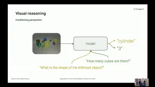
Okay,
let's
switch
over
to
a
new
example,
visual
reasoning.
So,
very
briefly,
what
visual
reasoning
is
is
that
we
have
an
image
that
we
have
as
input
here,
and
we
want
to
ask
questions
about
that
image.
Any
questions
that
probe
the
models,
ability
to
reason
about
the
content
and
relationship
of
objects
between
between
objects
in
the
image.
B
So
what
I
mean
by
this
is
that
there's
there's
one
image
as
input,
but
we
could
ask
many
different
questions
about
it
and
our
goal
is
to
extract
the
right
kind
of
information,
so
the
image
needs
to
be
processed
in
the
context
of
that
question
note
here
that
we're
not
limited
to
a
finite
set
of
contexts
like
the
finite
set
of
classes
in
our
class,
conditional
generative
modeling
example,
because
for
any
input
image,
there's
an
unbounded
number
of
questions.
We
could
ask
about
that
image
from
the
multitask
learning
perspective.
B
One
question
amounts
to
one
computational
process.
What
I
mean
by
this
is
a
question
we
could
ask.
I
could
apply
to
any
input
image,
assuming
of
course,
that
the
question
makes
sense
for
that
input
image.
So,
in
a
sense,
a
question
can
be
thought
of
as
a
task
description.
So,
for
example,
the
question
how
many
green
cubes
are.
There
corresponds
to
the
task
of
identifying
and
counting
green
cubes
in
an
image.
B
A
note
here,
more
generally,
about
visual
reasoning
is
that
it's
not
enough
to
do
well
to
do
well
on
the
previous
tasks
that
we've
seen
so
questions
in
the
training
set,
because
to
be
useful.
A
visual
reasoning
model
should
be
able
to
generalize
to
new
questions
and
there
is
no
training
data
that
exists
for
those
questions.
We
don't
have
a
paired
input
and
output,
and
so
there's
a
name
for
that
problem.
It's
called
zero
shot
learning
and
the
reason
why
it
could
ever
work
is
because
we're
exploiting
similarities
between
tasks.
B
B
So
if
the
model
is
able
to
answer
these
two
questions,
then
perhaps
it's
in
a
good
position
to
answer
that
question
here,
but
to
build
a
useful
notion
of
task
similarity.
We
need
to
build
task
representations
and
a
task
representation
allows
us
to
project
those
task
descriptions
onto
a
space
in
which
distances
are
indicative
of
similarity
between
tasks.
So
this
is
a
form
of
task
representation.
B
B
Okay,
so
to
summarize,
I've
introduced
a
few
different,
complementary
perspectives
on
some
learning
problems
and
the
common
denominator
for
these
perspectives
is
a
requirement
to
combine
different
information
sources,
and
that
goes
beyond
the
usual
input-output
data
processing
paradigm
of,
for
instance,
supervised
learning.
So
next
we'll
examine
one
family
of
approaches
to
combining
these
different
information
sources,
which
I
call
feature
wise
transformations
and
we'll
examine
how
these
different
learning
perspectives
fit
into
the
framework
of
feature
wise
transformations.
B
In
short,
it's
a
transformation
on
an
input,
feature
vector
or
a
stack
of
feature
Maps
that
acts
independently
on
individual
features
or
feature
map,
so
I'll
get
to
the
feature
map
in
convolutional
case
in
just
the
next
slide,
but
for
now
let's
concentrate
on
the
vector
case.
So
what
I
mean
by
that
is
that
we
have
an
input
which
is
a
vector
and
then
we
have,
for
instance
we
could.
We
could
bias
it.
So
we
have
a
biasing
vector
and
then
the
operation
is
applied,
element
wise
on
each
features,
so
we're
not
recombining.
B
Those
features,
we're
not
taking
weighted
sums
of
those
features
were,
for
instance,
biasing
them
individually
or
scaling
them
individually.
We
could
also
be
gating
them,
so
if
the
scaling
is
restricted
to
be
between
0
&
1,
we
have
a
sort
of
soft
on/off
kind
of
semantics,
so
that
could
be
achieved
by
passing
our
scaling
vector
through
a
sigmoidal
activation
function,
for
instance,
and
we
can
generalize
all
of
these
three
examples
into
a
notion
of
feature
wise,
affine
transformation.
So
in
in
a
visual
reasoning,
paper
I,
co-authored.
B
B
Okay
and
and
future
wise
transformations
are
used
quite
a
lot
as
you'll
see,
so
it's
kind
of
useful
to
have
a
catch-all
turn
to
reason
about
them,
so
something
that
is
either
scaling,
shifting
gating
anything
of
that
nature.
So,
in
this
lecture,
we'll
use
the
film
nomenclature
and
the
reason
for
that
is
because
I
think
it's
a
useful
communication
tool.
As
I
said,
it's
a
catch-all
term.
B
It
allows
us
to
reason
more
abstractly
about
these
concepts,
but
please
don't
take
this
as
me,
claiming
technical
innovation
and
all
of
these
methods
that
I'll
be
discussing
because
many
papers
out
there,
some
of
which
predate
the
film
lament
lecture,
make
use
of
feature
wise
transformations.
So
it's
more
of
an
observation
on
the
the
fact
that
these
sorts
of
approaches
are
pretty
ubiquitous,
depending
on
the
restrictions
that
we
impose
on
these
film
permit
parameters,
so
the
scaling
and
shifting
coefficients
we
we
recover
different
flavors.
B
So
if
there
are
no
restrictions,
we
recover
just
film
if
the
the
scaling
is
forced
to
be
one,
we
recover
biasing.
If
the
biasing
is
forced
to
be
zero,
we
recover
scaling
and
then,
as
I
said
earlier
or
skeptic
the
scaling
to
be
between
0
&
1.
We
get
a
so
here's
an
example
animation
showing
how
this
works.
So
we
have
an
input
vector
and
then
we
can
control
the
value
of
the
scaling
and
shifting
coefficients,
and
you
see
that
they
only
affect
one
feature
here.
B
So
this
is
why
we
call
this
feature
wise
transformations,
okay,
so
in
the
convolutional
case
that
I
brushed
aside
earlier,
the
way
this
works
is
that
we
still
have
one
scalar,
but
one
scalar
and
out
per
feature
map
and
and
the
the
reason
for
that,
in
short,
is
because
you
can
think
of
the
convolution
operation
as
involving
a
feature
detector
over
different
spatial
positions.
So
so
in
essence,
the
feature
map
represents
the
same
feature
but
evaluated
at
different
spatial
positions.
B
So
from
that
perspective
it
sort
of
makes
sense
that
we
would
want
to
scale
and
shift
entire
feature
Maps
rather
than
different
spatial
positions.
But
there
are
papers
out
there
that
untie
this
scaling
and
shifting
to
different
spatial
positions,
and
there
are
situations
in
which
that
makes
sense.
So
it's
more
of
a
rule
to
be
broken
than
just
a
statement
about
all
of
these
methods.
B
All
right,
so
we
introduce
feature
wise
transformations
to
the
model
by
inserting
film
layers.
So
these
these
things
here
that
I
showed
in
just
the
last
slide
into
an
existing
network
architecture,
so
everything's
trained
jointly.
It's
just.
We
update
the
network
architecture
by
inserting
these
film
layers
and
we'll
call
the
scaling
and
shifting
coefficients
here.
The
film
parameters
in
our
nomenclature
and
to
reiterate
film
layers
here
are
an
abstraction,
so
they
can
mean
either
of
feature-wise,
affine,
biasing
scaling
or
gating
transformations.
B
Let's
make
this
concrete.
So
let's
revisit
the
class
conditional
generative
modeling
example,
so
the
feature
wise
transformation
approach
to
building
a
class
conditional
model
here
would
be
to
start
with
an
unconditional
model
and
then
turn
it
into
a
a
class
conditional
model.
So
just
reminder
of
the
problem
why
we
want
to
do
this
is
because,
if
we
are
to
learn
separate
generators
for
each
class
in
the
data
set,
we
have
an
explosion
in
the
number
of
trainable
parameters,
and
we
want
to
avoid
that.
B
B
Okay,
let's
Quinn
our
eyes
again.
There
are
different
ways
of
explaining
what
we're
doing
here.
One
interpretation
is
that
this
is
a
fancy
and
come
back
to
way
of
describe
severals
class-specific
generators
would
just
which
just
happen
to
share
most
of
their
parameters.
So,
in
other
words,
we
have
different
generators
here
that
are
not
explicitly
represented,
but
we
can
think
of
them
implicitly,
and
so
they
share
all
of
these
parameters
here
and
they
specialize
these
sets
of
parameters
in
the
network,
and
so
what's
really
going
on
when
we're
conditioning.
B
Is
that
we're
implicitly
swapping
out
class
specific
generators?
So
that's
one
interpretation.
Another
interpretation
is
that
this
is
a
special
kind
of
a
hyper
network.
So
for
those
of
you
who
don't
know
what
a
hyper
network
is
it's
a
network
which
predicts
the
parameters
for
another
network,
so
what's
going
on
here,
really
is
that
we're
we're
taking
the
cat
class
we're
feeding
it
through
our
hyper
network,
which
will
predict
the
value
for
the
film
parameters,
and
then
we
can
feed
in
the
noise
and
get
the
output
as
a
result.
B
So
one
way
to
use
feature
wise
transformations
for
this
is
to
start
with
a
convolutional
Network.
So
we're
still
trying
to
map
an
input
to
perhaps
a
distribution
over
possible
answers
and
like
what
the
class
conditional
generator
will
insert
film
layers
throughout
the
architecture,
but
here,
instead
of
learning
a
separate
set
of
film
parameters
per
class
because,
as
a
reminder,
there's
an
unbounded
number
of
questions
we
can
ask.
B
So
we
can't
really
learn
a
separate
set
of
film
parameters
for
each
will
will
learn
a
mapping
from
the
question
itself
to
the
value
of
the
film
parameters.
So
here
I
could
use,
for
example,
a
recurrent
neural
network
to
map
the
the
question
to
the
value
of
the
film
parameters
and
just
as
a
side
note,
this
is
far
from
the
only
approach
to
visual
reasoning
out
there.
B
There
are
some
approaches
that
incorporate
additional
inductive
biases,
such
as
a
notion
of
modularity
in
the
visual
pipeline
like
I,
want
to
be
composing,
explicit
blocks
of
computation
or
are
they
can
also
Inc
operate
a
notion
of
relation
between
objects?
So
this
is.
This
is
not
the
only
way
to
solve
the
problem,
but
it
is
a
way
which
doesn't
have
a
lot
of
inductive
bias
suspected
to
it.
B
Ok,
let's
move
away
from
problem
specific
details
and
consider
an
abstraction
that
fits
both
the
class
conditional,
generative
modeling
problem
in
the
visual
reasoning
problem.
So
in
both
cases
we
have
two
components
to
the
model
architecture.
We
have
a
task
solving
Network
being
modulated,
which
we'll
call
the
film
Network,
and
we
have
an
auxiliary
Network,
which
Maps
a
task
description
to
a
set
of
modulation
parameters
which
we'll
call
the
the
film
generator
here.
So
the
film
generator
can
be
really
simple
or
complex.
B
In
the
class
conditional
generative
modeling
example,
we
saw
that
it
was
just
selecting
parameters,
so
you
can
think
of
this
as
we're
building
a
big
matrix
of
film
parameters.
The
rows
represent
different
classes
and
the
columns
represent
different
scaling
and
shifting
coefficients
for
different
features
or
feature
maps,
and
so
the
film
generator
really
is
just
selecting
a
row
in
that
matrix
and
using
the
parameter
values
inside
of
the
network.
B
So
one
modular
one
modality
is-
is
influencing
how
another
one
is
being
processed
as
opposed
to
the
two
modalities
being
processed
in
parallel
for
some
time
and
then
aggregated
for
further
processing,
as
we
continue
in
the
lecture,
I'll
become
less
and
less
perspective
agnostic
and
rely
more
heavily
in
the
conditioning
perspective,
and
the
reason
for
that
is
because
I
think
there
are
interesting
observations
and
insights
to
explore
here.
But
in
my
that
there
is
merit
to
all
perspectives,
and
sometimes
the
modality
fusion
perspective
is
more
suitable.
B
So,
for
instance,
what
happens
if
we
have
three
modalities
which
we
want
to
combine
together?
How
would
we
use
the
film
framework
for
that
not
clear
or
what
happens
if
I
have
two
modalities,
for
instance
audio
and
video,
in
a
video
clip
which
don't
have
a
clear
conditioning
relationship?
Once
again,
it's
it's
a
bit
harder
to
think
about
this
from
the
conditioning
perspective.
B
Okay,
at
this
point,
I
think
it
would
be
useful
to
over
to
go
over
a
few
example.
Applications
and
the
goal
here
is
to
help
you
recognize
applications
of
feature
wise
transformations
in
the
literature
and
as
you'll
see,
they
come
with
many
different
names.
So
it's
good
to
be
able
to
connect
them
back
to
a
more
general
framework
and
I
also
want
to
get
you
to
draw
parallels
with
your
own
problems.
B
Perhaps
you'll
recognize
something
useful
for
you
and,
as
such,
I'll
be
focusing
on
showing
different
aspects
of
feature
wise
transformations,
so
I
won't
be
necessarily
thorough
in
citing
all
of
the
relevant
literature.
I
won't
be
doing
justice
to
the
full
history
of
application
of
feature
wise
transformations
and
in
the
distal
article.
We
also
have
this
this
sort
of
recency
bias,
but
we
do
have
bibliographic
notes
that
attempt
to
be
a
bit
more
thorough
in
pointing
to
older,
related
work.
So
if
you're
curious
about
that,
I
would
encourage
you
to
check
out
the
de
Soto
article.
B
Okay,
let's
start
with
a
straightforward
one.
So
this
is
the
visual
reasoning.
Example
I
gave
earlier,
and-
and
this
is
the
paper
in
which
we
proposed
the
film,
the
language
er,
and
so
there's
not
much
else
to
say
about
this.
So
in
this
specific
case
we're
inserting
film
layers
in
the
residual
blocks
of
the
network.
But
aside
from
that,
I
think
you
get
the
you
get
the
picture.
B
Feature
wise
transformations
have
also
been
applied
to
style,
transfer
and
we'll
see
three
examples
of
that,
so
small
primer
on
style
transfer,
if
you're
not
familiar
so
some
approaches
to
style,
transfer,
train
a
feed-forward
network
that
is
specialized
single
stamina.
So
the
idea
here
is
I
have
a
style
image.
I
have
a
content
image
I
want
to
produce
a
pastiche,
a
stylized
version
of
the
content
image
in
the
style
of
this
image.
How
do
I
do
that?
Well,
I
specialize.
B
My
network
I
fix
the
style
image,
I
specialize
my
network
to
to
that
style
image
and
then
I
train
a
network
which
is
able
to
turn
any
input
content
image
into
its
best
dish
of
that
specific
style.
The
the
loss
formulation
is
unimportant
for
this
discussion,
so
just
know
that
there's
a
way
to
provide
a
training
signal
that
encourages
that,
and
here
we're
also
faced
with
an
explosion
in
parameters,
because,
if
I
train
a
special
network
for
each
style,
image
and
I
want
to
build
a
system
that
is
a
collection
of
different
style
images.
B
Well,
I
need
to
train
separate
networks
for
each
each
style
image.
So
again,
the
naive
approach
that
trains,
one
network
per
style
image
in
this
system,
leads
to
an
explosion
in
the
number
of
parameters
that
you
need
to
train
and
so
again
the
the
feature
wise
transformation
solution
to
that
is
to
turn
the
network
into
a
style
conditional
version
of
itself
by
inserting
film
layers
in
the
network
architecture.
Okay,
so
let's
examine
these
three
examples.
B
The
first
example
is
a
paper
I
authored,
where
we
were
considering
a
setting
in
which
we
have
a
finite
collection
of
style
images.
So
this
is
very
similar
to
the
class
conditional
generative
modeling
example,
but
instead
of
having
classes
to
to
model,
we
have
different
styles
to
model
and
and
the
intuition
behind
that,
or
really
was
that
we
wanted
somehow
to
compress
these
many
different
models
into
one
style
conditional
model.
B
We
want
it
to
be
more
parameter,
efficient
and
the
way
in
which
we
do
the
conditioning
is
by
specializing
instance,
nominalization
layers
in
the
network
to
each
style,
so
small
modem
on
that
normalization
layers
are
a
natural
location
to
use
feature
wise
transformations,
because
so
just
small
reminder
on
on
normalization
layers.
So
you
you
take
your
input,
feature
vector
or
stack
of
feature
Maps,
you
normalize
it
with
respect
to
the
whole
batch
or
spatial
axes
or
whichever
variant
you
want,
and
then
you
have
a
scaling
and
a
shifting
operation
afterwards
to
control.
B
B
B
Okay,
so
we
can
extend
that
pretty
naturally
to
the
zero
shot.
Setting
so
say,
I
have
a
new
style
image.
My
system
wasn't
trained
on
it,
I'd
like
to
be
able
to
do
well
on
that.
Well,
as
we
seen
with
the
the
visual
reasoning
example,
we
can
do
so
by
predicting
film
parameter
values
from
the
task
description.
So,
in
this
case,
our
task
description
is
the
sound
image.
Well,
why
not
introduce
a
mapping
from
style
image
to
film
parameter
values,
so
this
is
what
was
done
in
this
paper
and.
B
B
The
film
generator
predict
a
set
of
film
parameters
to
be
used
in
the
main
style
transfer
Network,
and
then
we
feed
in
the
content
image,
and
then
we
get
the
output-
and
this
is
a
small
animation
here
to
show
you
what
happens
if
you
V
feed
in
style
images
that
have
not
been
seen
during
training
and
as
you
can
see,
the
model
does
a
pretty
good
job
at
zero
stretch.
Generalization
in
this
case.
B
Another
related
example
that
you
might
see
cited
in
other
papers
is
a
des
in,
for
adaptive
instance
normalization.
This
is
yet
another
name,
but
the
principle
stays
the
same.
We
specialize
incidence,
normalization,
parameter
values
to
different
style
images,
and
it
also
allows
you
a
generalization.
What
I
think
is
interesting
in
this
work
is
the
way
in
which
the
film
generator
is
constructed.
So
in
in
the
previous
work,
we
had
a
explicit
mapping
from
style
image
to
the
value
of
the
film
parameters
here.
B
What's
happening
is
that
we
feed
both
the
content
in
the
style
image
through
some
encoder
that
is
shared
between
the
two
and
then
when
we
want
to
perform
instance
normalization.
We
normalize
the
content,
stack
of
feature
maps
and
then
we
scale
it
and
shifting,
according
to
statistics
collected
from
the
style,
stack
of
feature
maps
and-
and
that
is
sufficient
in
their
case,
to
allows
your
shot
generalization.
So
if
you
squint
your
eyes
again,
the
film
generator
is
a
heuristic
that
reuses
the
encoder
networking
and
performs
a
fixed
processing
on
this
town
stack
of
future
maps.
B
Okay,
this
problem
setting
should
be
familiar
to
you.
We're
talking
about
class
conditional,
generative
modeling
has
Emily
discussed
began
yesterday,
maybe
maybe
not
yes,
I
have
a
yes
good,
so
I
won't
spend
too
much
time
talking
about
it
again.
This
is
a
pretty
impressive
model
that
came
out
recently
and
it
uses
conditional
batch
normalization
for
class
conditioning
which
you'll
recognize
as
an
application
of
each
OS
transformations.
B
It
also
incorporates
a
twist
on
how
the
generator
uses
the
input
noise,
so
a
low
dimensional
embedding
is
learned
for
each
class
and
then
the
the
way
in
which
we
predict
the
film
parameters
is
that
so
first
we
take
the
noise
vector
as
input
and
we
chunk
it
into
different
different
chunks.
So
this
is
what's
in
here,
so
we
take
that
as
input.
We
split
it
into
different
chunks,
which
are
our
here,
and
then
we
concatenate
the
noise
chunk
to
the
class
embedding,
and
then
we
linearly
project
that
into
some
parameter
values.
B
So
one
way
to
see
this
is
that
noise
is
being
injected
at
multiple
locations
in
the
generation
process.
Another
way
to
see
this
is
that
we
have
noisy
film
parameter
values
and,
and
that,
as
you
can
see
on,
the
right
allows
to
generate
pretty
convincing
images.
Of
course,
this
is
not
the
only
ingredient
in
there
that
makes
it
work.
They
scaled
the
architecture
up
by
quite
a
lot
scaled
up.
The
batch
size
as
well,
but
but
feature
wise
transformations
are
at
the
core
of
the
class
conditioning
mechanism.
B
This
work:
okay,
let's
travel
back
to
the
ancient
times
of
2015-2016,
which
by
deep-learning
years,
is
really
really
old.
Apparently,
so
this
again
is
perhaps
the
most
cited
Gantt
paper
after
the
original
yawn
paper,
because
it
introduced
a
convolutional
architecture
that
worked
much
much
better
than
the
fully
connected
architecture
in
the
original
Gantt
paper
and
the
condition
on
the
class
by
concatenating
the
class
label
two
stacks
of
feature
maps
in
the
network.
So
it's
a
slightly
different
mechanism.
B
They
do
conditioning
by
concatenation
rather
than
by
biasing,
but
the
reason
why
I
point
out
this
paper
to
you
is
because
there's
an
equivalence
between
concatenation,
based
conditioning
and
and
conditional
biasing,
and
the
reason
why
so
think
of
think
of
this
example
here.
So
we
have
our
input
here
and
we
have
the
conditioning
signal
here.
We
can
catenate
them
together.
B
We
multiply
that
with
a
matrix,
you
can
always
decompose
the
matrix
vector
product
into
two
smaller
products,
one
with
just
the
input
and
one
with
just
a
conditioning
signal,
and
afterwards
you
add
the
these
two
resulting
vectors
element
wise,
and
what
you
can
recognize
here
is
that
you
can
think
of
this
as
a
conditioning
bias.
So
really
concatenation
and
biasing
are
essentially
the
same
from
that
point
of
view.
B
Why,
while
we're
on
the
topic
of
Ganz,
here's
another
recent
architecture
which
made
quite
a
splash,
it's
called
style,
yawn
and
those
are
actual
model
samples,
not
they're,
not
real
pictures
of
faces.
So
it
did
very
well
on
that
task,
and
one
of
the
central
principles
here
is
that
the
input
noise
vector
is
it
isn't
even
fed
as
input
to
the
generator.
B
B
So
that,
but
that
is
another
twist
on
how
to
use
feature
wise
transformations
and
and
they
they
even
removed
the
input
from
the
generator
in
that
Chase.
Okay,
so
switch.
Let's
switch
gears
a
little
here's
another
cool
idea,
so
say
that
you
want
to
deploy
a
model
on
devices
that
have
different
amounts
of
processing
power.
You
could
train
separate
networks
with
different
widths
for
it,
for
example,
to
have
different
kind
of
computational
expenses.
B
If
you
will
one
for
each
desired
level
of
computational
effort,
but
as
we
discussed
in
the
context
of
class
conditional
generative
modeling,
this
is
wasteful,
and
so
instead
it
we.
It
would
be
better
to
train
a
single
network
and
use
only
the
neurons
up
to
a
certain
width
in
the
network.
So
you
can
deploy
only
one
model
and
then
you
can
select
the
width
that
you
want
to
use
that
corresponds
to
the
computational
effort
you
want
to
make.
B
It
turns
out
that
by
specializing
batch
normalization
layers
to
each
Stargate
with
which
they
call
switchable
batch
normalization
in
the
paper,
you
can
do
just
that.
So
the
idea
is
that
we
learn.
So
there
are
Bachelor
mobilization
layers
in
this
model
architecture
and
then
we'll
learn
different
sets
of
parameters
for
each
width,
and
it
turns
out
that
you
can
get
good
good
accuracy
and
computational
effort
trade-offs,
and
you
can.
You
can
select
the
width
at
at
deployment
time.
B
Okay,
so
far,
we've
only
covered
image,
synthesis
applications
but
feature
wise
transformations
are
also
used
in
other
research
areas.
So
here's
the
reinforcement,
learning
example
and
the
goal
here
is
to
do
instruction
following
so
we
have
an
agent
here
which
is
navigating
in
in
a
do
like
environment,
and
we
have
an
instruction
and
we
expect
the
agent
to
carry
out
that
instruction
and
the
instruction
is
in
the
natural
language.
So
in
this
example,
the
way
in
which
the
policy
network
is
conditions
is
that
we
predict
feature
wise,
gating
parameters
from
the
instruction.
B
So
we
have
the
instruction
as
input
we
process
it.
And
then
we
predict
gating
parameters
to
be
applied
to
the
output
of
the
visual
pipeline
part
of
the
policy,
and
in
that
paper
it
is
sufficient
to
be
able
to
the
instruction
following
here.
We
have
a
language
model
where
one
half
of
the
feature
vectors
is
used
to
predict
how
to
get
the
other
half.
So
in
this
diagram.
B
So
the
motivation
in
this
paper
has
more
to
do
with
avoiding
gradient
vanishing.
Then
it
has
to
do
with
using
few
choice,
transformations
but
I
think
it's
it's
illustrative
of
another
interesting
concept
here,
which
is
that
of
self
modulation.
So,
in
the
examples
I
gave
previously,
the
conditioning
signal
was
always
external.
B
B
So
this
is
the
submission
that
won
the
first
place
in
the
image
net.
2017
challenge,
and
one
of
the
central
ideas
in
the
model
architecture
is
that
they
have
a
pathway
branching
off
from
the
main
pathway,
and
that
is
predicting
feature,
wise
scaling
parameters
to
be
applied
onto
the
main
pathway
and
and
that
architectural
feature,
along
with
the
other
improvements
suggested
in
the
in
the
paper,
helped
win
this
image.
A
20-17
competition.
B
Okay,
so
somewhat
related
to
self
modulation
is
the
idea
of
adapting
to
changes
in
the
input
distribution.
Oh
here's
an
example
illustrating
that
here
we
have
a
speech,
recognition
model
and
we
we
want
it
to
be
robust
to
different
speakers
and
to
different
noise
conditions,
and
so
the
way
in
which
this
model
does
it
it
that
it
first
builds
a
representation
of
the
full
utterance
and
then
it
uses
that
to
predict
layer,
normalization
parameter
values
to
be
used
inside
of
the
linear
layer,
normalization
layers.
B
They
call
that
dynamically
your
normalization
in
this
paper,
but
again
it's
an
instance
of
feature
wise
transformation
and
here's.
Another
example
of
that.
So
the
this
notion
of
adapting
to
different
input
distributions
using
few
choice
transformations.
We
also
find
it
in
fuchsia
image
classification.
So,
very
briefly,
what
is
few
shots
image
classification,
so
few
shot.
Learning
aims
to
learn
from.
B
Okay,
okay,
so
hopefully
these
examples
give
you
a
good
taste
at
the
variety
of
settings
in
which
feature
wise
transformations
are
applied.
Now,
I'd
like
to
focus
on
interesting
properties
of
feature
wise
transformations
themselves
and
I'll
start
with
a
disclaimer.
Some
of
the
interpretations
that
I'll
be
making
in
this
part
of
the
lecture
are
more
speculative
than
factual
by
nature.
So
please
do
exercise
critical
thinking
assessing
what
I'm
saying
here.
B
Okay,
one
interesting
consequence
of
film
is
that
we
end
up
predicting
a
low
dimensional
vector
of
film
parameters,
and
so
to
give
you
an
example
in
the
style
transfer
model,
I
was
working
on
the
the
number
of
film
parameters
accounted
for
about
point.
Two
percent
of
the
total
parameter
count
in
the
in
the
whole
model.
So
that's
not
a
lot
of
parameters
to
be
modulating
to
have
such
a
drastic
effect
on
the
computational
properties
of
the
model,
so
squinting
our
eyes
again.
There's
at
least
two
possible
interpretations
to
this.
B
One
from
the
computational
perspective
is
that
film
parameters
are
an
instruction
on
how
to
modulate
computation
in
the
task
solving
Network.
Another
interpretation
from
the
representation
learning
perspective
is
that
film
parameters
are
a
representation
of
the
task
description.
So,
let's
focus
on
the
representation
learning
perspective
for
an
instant
so
assume
we
can
extract
a
representation
from
our
task
descriptions.
What
can
we
do
with
that
representation?
B
B
Now
my
background
is
in
generative
modeling
and
we
have
a
cliche,
which
is
that
we
love
to
do
interpolations
in
latent
space.
So
we
love
to
interpolate
Victor's
in
latent
space
and
see
things
very
smoothly
in
pixel
space,
and
this
is
a
bit
like
when
the
neural
networks
community
was
fixated
and
showing
wait
filters
for
a
while.
So
we
have
that
vishay,
I
guess
and
of
course,
when
I
was
working
on
south
transfer
I
had
to
interpolate
film
parameters.
B
So
here's
what's
going
on
in
this
animation,
each
individual
image
on
the
Left
corresponds
to
a
different
style
that
the
model
was
trained
on
and
to
the
right.
Here
we
have
the
feed
of
a
camera,
video
feed
of
a
camera
that
is
being
fed
through
the
style,
transfer
network
frame
by
frame
and
then
we're
using
the
film
parameters
that
you
know
describe
how
we
get
them
afterwards
and
the
to
stylize
a
simile.
And
so
how
do
we
get
these
film
parameters?
B
There's
a
pretty
clear
use
case
in
this
example:
it's
a
more
natural
way
of
interacting
with
the
model.
It
allows
users
to
blend
Styles
together
to
express
our
creativity,
but
I
think
that
I'm
at
a
more
abstract
level.
What
we
can
conclude
from
that
is
that
interpolating
between
tasks
refers
representations
leads
to
meaningful
changes
to
the
task,
solving
networks,
computational
properties.
So
this
is
not
a
property
that
should
hold
in
all
use
cases,
but
in
this
instance
it
does,
and
it
also
does
in
this
example.
B
So
this
is
Big
John
again
and
as
a
reminder,
this
is
a
class
conditional
generative
model
where
we're
conditioning
by
a
film
layers
inserted
throughout
the
architecture,
and
so
the
and
the
film
parameters
are
predict
predicted
linearly
from
the
concatenation
of
the
input
noise
and
a
learn
class.
Embedding
a
consequence
of
doing
things.
That
way
is
that
we
now
have
a
class
representation
for
each
class
and
we
can
think
of
interpolating
between
these
class
representations.
B
So
we
can
probe
what's
in
between
categories
by
taking
linear,
interpolations
of
class
and
Eddings,
and
once
again
you
see
smooth
transitions.
It
kind
of
reminds
me
of
the
old
Animorphs
TV
show
for
those
of
you
who
know
what
I'm
talking
about
and
what's
interesting
here
as
well,
is
that
the
the
post
remains
roughly
the
same
in
those
examples
which
maybe
suggest
that
there's
a
nice
separation
between
what's
encoded
by
the
input
noise
and
was
encoded
by
the
class
embeddings.
B
So
they
said
bility
to
interpolate
between
tasks
sighs
in
light
nicely
with
the
brother
theme
of
what
meaning
to
assign
to
hidden
layers
in
a
neural
network,
as
you've
probably
been
told.
One
interpretation
is
that
a
hidden
layer
is
an
abstract
representation
of
the
input,
but
an
alternative
interpretation
which
I
first
heard
from
Ian
Goodfellow,
but
almost
certainly
it's
been
put
forward
by
others-
is
that
hidden
layers
amount
to
intermediate
stages
in
a
numerical
program.
B
So
what
this
suggests
to
me
is
that
feature
wise
transformations
may
be
a
mechanism
through
which
a
model
learns
and
composes
computational
primitives,
and
this
interpretation
is
closer
to
the
computational
perspective
than
the
representation
learning
perspective.
But
as
you've
noticed
by
now,
moving
freely
between
interpretations
is
more
or
less
a
theme
of
its
own.
In
this
lecture,
so
I
think
this
is
a
good
thing.
B
Ok,
beyond
interpolation
is
another
operation
that
the
deep
learning
community
loves
to
apply
to
representations
is
analogies.
So
here
we
have
the
classical
word
to
Veck
example.
So
in
word
two
that
we
learn
and
embedding
forwards
in
a
vocabulary,
and
then
we
perform
analogies.
So
the
classical
example
is
King.
Man
plus
woman
was
Queen,
and
so,
if
we
take
the
word
embedding
for
the
word,
King
subtract,
the
one
for
the
word
man
add
the
one
for
the
word
woman
low
and
behold
we
get
the
embedding
for
the
word.
Queen
terms
and
conditions
apply.
B
You
have
to
exclude
the
query
words
here
for
that
to
work,
but
you
get
the
idea.
So
in
our
visual
reasoning,
work
we
were
curious
to
see
if
that
property
also
held
for
the
learned
task
representations.
So
in
this
example,
the
question
is
what
is
the
blue
big
cylinder
made
of,
and
so
the
usual
way
of
operating
the
model
is
that
we
feed
the
question
through
the
film
generator.
We
use
the
output
film
parameters
in
the
task
solving
Network
and
we
feed
in
an
input
image.
B
We
get
a
predicted
answer
as
output
in
this
case
rubber,
which
is
not
the
right
answer.
It
should
be
now,
and
perhaps
this
is
because
the
question
involves
concepts
that
have
have
been
seen
in
training,
but
in
nice
elation
never
together
before
so
the
model
doesn't
really
know
what
to
do
with
it.
With
that
new
question,
but
in
any
case
what
happens
here
is
that
the
model
fails
to
generalize
to
a
new
question.
B
So
taking
inspiration
from
the
word
cubic
examples,
an
alternative
way
of
operating
the
model
is
to
express
this
question
here
as
a
combination
of
three
questions
that
have
been
seen
during
training.
So
the
question:
what
is
the
blue
big
cylinder
made
of
can
be
thought
of
as
what
is
the
blue
big
sphere
made
of
plus?
What
is
the
green
big
cylinder
remain
of
what
is
the
green
big
sphere
made
of
so
in?
B
B
So
first
we
feed
all
these
three
questions
through
the
film
generator.
Then
we
combine
their
film
parameters
in
the
same
way
and
it
turns
out
that
this
works
for
visual
reasoning
or
for
the
visual
reasoning
model.
We
were
studying
not
always,
but
it's
still
corrected
a
non-negligible
amount
of
errors
that
the
model
was
making.
So
I
think
this
is
an
interesting
observation
and
it's
own,
but
it
also
raises
interesting
questions
about
failure
modes
for
this
type
of
architecture.
B
More
generally,
the
film
sort
of
framework,
so
knowing
that
we
can
recover
the
right
answer
through
algebraic
manipulations
of
film
parameters
when
a
model
makes
a
mistake,
is
it
because
it
lacks
computational
primitives
to
solve
the
task?
Or
is
it
because
it
failed
to
combine
them
appropriately
and
I?
B
So
if
you're
ever
working
with
these
types
of
architectures
know
that
there
are
many
sources
of
overfitting
and
and
know
that
you
can
target
different
parts
of
the
architecture
to
combat
that
another
lesson
to
be
learned:
oh
yes,
I!
So
so
I!
It's
a
good
question,
I!
Think!
If
you're,
if
you're
primed
on
the
problem,
you
could
probably
answer
that
question
correctly.
So
here
the
the
the
rubber
objects
are
never
shiny,
so
they're
there
math,
and
so
so.
This
is
a
way
in
which
so
this
is
this
is
an
artificially
constructed.
B
Setting
I'd
say
this
specific
data
set
clever
was
was
built
because
it
was
observed
that,
in
visual
reasoning,
the
models
turned
tended
to
rely
on
biased
season
the
data
set
rather
than
on
actual
reasoning
capabilities.
So,
if
I
asked
you,
if
you
see
a
green
pasture
and
I
asked
you
what
is
the
animal,
you
probably
think
this
is
a
cow,
and
this
is
exactly
what
the
model
was.
The
models
were
doing.
They
were
not
answering
based
on
the
content
of
the
image,
but
just
based
on
the
statistical
similarities.
B
So
the
goal
for
that
specific
data
set
was
to
reduce
these
sorts
of
biases
that
the
model
could
rely
on
now.
Is
it?
Is
it
a?
Is
it
a
fair
task
to
be
achieved
by
humans,
I?
Think
humans
were
scoring
pretty
well
when
they
were
evaluated
on
that
I'd
have
to
look
again.
Maybe
it's
that
specific
example,
that
is,
that
is
confusing,
but
generally
we're
pretty
good
for
that
Addison
as
well.
B
So
the
other
lesson
so
again
getting
back
into
into
the
context.
So
why
are
we
waking
making
mistakes
and
and
what
lessons
this
can
can
tell
us.
So
another
lesson
is
that
the
film
point
of
view
I
think,
highlights
a
separation
between
the
various
computational
primitives
that
are
learned
by
the
film
Network.
So
these
are
the
computational
primitives.
If
you
will,
and
the
numerical
rest
recipes,
that
we
learn
through
the
film
generator
and
how
to
combine
those
computational
primitives.
B
Okay,
I'd
like
to
conclude
this
lecture
by
discussing
notions
of
interpretability
I'm
by
no
means
an
expert
on
the
topic
and
luckily
you'll
get
to
hear
from
an
actual
expert
on
the
topic
right
after
the
break.
But
I
couldn't
pass
on
the
opportunity
to
discuss
what
sort
of
interpretations
we
can
make
in
the
context
of
a
choice
transformations
so
when
I
was
playing
with
conditional
instance,
normalization
in
the
sound
transfer
work.
B
One
of
the
things
that
surprised
me
very
much
is
that,
despite
their
simplicity,
feature-wise
transformations
are
very
effective
at
modulating
the
computation
in
a
network
again
point
two
percent
of
the
total
parameter
count
that
we're
varying
that
is
sufficient
to
cause
drastic
changes
in
the
computational
properties
of
the
style
transfer
network
and
it's
been
I.
This
is
the
hammer
I've
been
hitting
every
nail
with
ever
since
and
it's
it's
been
pretty
effective
in
many
different
problem
settings.
B
B
B
So,
for
instance,
we
could
think
of
feature
wise
transformations
as
a
mechanism
for
shutting
up
features
or
feature
nots,
and
and
why
would
that
be
a
selection
mechanism?
Well,
if
you
take
a
feature
and
you
zero
it
out,
it's
as
if
you
had
never
computed
it
in
the
first
place,
so
you
could
do
it
by
setting
the
scaling
to
zero
and
the
biasing
to
zero
as
well.
You
could
do
it
by
using
a
very
negative
bias.
B
So
if
your,
if
your
operation
is
followed
by
some
non-linearity,
which
zeros
out
things
that
are
negative
like
rectified
in
your
unit,
for
instance,
that
could
be
that
could
be
used.
So
maybe
there
is
a
mechanism
like
that
at
play
here,
and
it
sounds
like
a
wonderful
interpretation,
but
in
practice
it
doesn't
hold.
B
So
one
of
the
things
we
would
expect
to
see
if
we're
selecting
features
left
and
right
is
that
applying
film
should
lead
to
a
non
negligible
amount
of
future
maps
that
are
turned
off.
However,
when
we
measure
the
sparsity,
we
found
it
to
be
very
low,
I
think
it's
at
most
10%
of
the
feature
maps
that
were
completely
off
at
any
given
time
and
in
instances
where
the
feature
maps
were
turned
off.
B
We
weren't
able
to
identify
a
unique
mechanism
which
would
explain
why
they
were
turned
off,
so
things
were
a
bit
all
over
the
place.
So
sadly,
the
conclusion
we
drew
from
this
is
that
there's
no
supporting
evidence
for
the
selection,
some
hypothesis
and
there's
apparently
no
unique
mechanism
by
which
film
can
turn
off
features
or
feature.
Maps
I,
wouldn't
completely
rule
out
a
modified
that
a
modified
version
of
the
hypothesis
could
offer
an
explanation
and
also
keep
in
mind
that
the
number
of
models
we
examined
is
extremely
small.
B
We're
talking
about
two
models
which
use
the
affine
bearing
and
so
there's
tons
of
things
to
explore
here,
but
to
this
day
I.
Don't
think
we
have
a
good
explanation
for
how
feature
wise
transformations
are
somehow
able
to
compound
into
meaningful
modulations
of
the
test.
Solving
Network
the
consolation
is
that
there
are
some
interesting
things
we
can
say
about
the
way
in
which
film
parameters
cluster
across
test
descriptions,
and
even
though
this
has
not
yielded
a
lot
of
insights
yet
into
how
film
operates
at
a
computational
level.
B
I
think
this
has
the
potential
to
help
interpret
the
purpose
of
different
parts
of
the
task
solving
Network.
So
let's
take
a
closer
look
at
that.
What
you
see
here
is
scatter
plots
of
film
parameters,
so
this
is
for
the
visual
reasoning
model.
This
is
for
the
sound
transfer
model.
The
x
axis
corresponds
to
the
scaling
coefficient.
The
y
axis
corresponds
to
the
shifting
coefficient
and
then
each
point
corresponds
to
a
different
task
description.
So
here
it's
a
different
question
here:
it's
a
different
style
image
and
then
also
a
different
feature
map.
B
B
So
mark
marginally
across
all
feature
maps.
This
is
a
big
mess,
there's
not
a
lot
of
structure.
But,
however,
if
we,
if
we
look
at
individual
feature,
Maps
so
individual
colors
here
we
see
that
there's
a
fairly
simple
structure
so
for
most
feature
maps
in
both
models.
The
points
tend
to
question
into
a
single,
dense
blob
and
for
the
visual
reasoning
model.
They
occasionally
form
more
than
so
wait
until
we
find
one.
So
this
one
this
one.
So
there
are
a
few
examples
like
that.
B
You
can
see
I'll
expend
more
on
that
later,
so
thinking
back
about
style
interpolations.
Maybe
this
explains
why
they
don't
produce
garbage
results,
because
any
convex
combination
of
some
parameters
is
likely
to
correspond
to
a
meaningful
parameterization
of
the
task,
solving
Network,
so
the
network
kind
of
knows
what
to
do
with
that.
So
that's
that's
reassuring.
B
Also,
looking
at
the
axis
alignment
of
those
different
blobs,
we
see
that
some
clusters
tend
to
vary
across
the
scaling
axis
like
in
this
example,
or
some
others
tend
to
vary
across
the
biasing
axis
and
some
tend
to
be
diagonally
aligned.
So
my
interpretation
of
this
is
that
the
model
has
learned
to
modulate
feature
maps
in
various
ways,
sometimes
by
a
scaling,
sometimes
by
a
biasing
and
sometimes
using
a
combination
of
both.
B
So
perhaps
when
we
were
looking
for
a
unique
mechanism
that
explained
how
film
modulates
it
was
a
bit
pointless,
there
are
many
mechanisms,
also
keep
in
mind.
This
is
for
affine
transformations,
I'm
sure
there
are
other
interpretations
to
make
in
the
case
of
gating,
for
instance,
or
other
types
of
mechanisms.
B
Okay,
so
those
film
primary
scatter
plots
hint
at
the
fact
that
the
way
in
which
film
parameters
are
structured
across
tasks
varies
depending
on
the
problem
setting.
So
this
is
what
I
was
sending
at
earlier
when
I
said
that
for
the
visual
reasoning
example,
we
see
more
than
one
modes
which
we're
not
observing
in
in
the
case
of
the
style
transfer
example.
B
So
this
means
that
perhaps
we
shouldn't
expect
to
find
a
unique
in
problem,
independent
explanation
for
the
success
of
feature
wise
transformations,
but
still
there
are
some
interesting
things
we
can
say
when
we
look
at
this
individual
problem,
so
I
am
showing
you
two
cherry-picked
examples
of
these
multimodal
blobs
that
we
found
in
the
visual
reasoning
model
and
in
in
the
distal
article.
We
hypothesize
that
maybe
this
the
compositional
indiscreet
nature
of
visual
reasoning
that
requires
these
different,
well-defined
modes
of
operation
that
are
not
necessarily
as
much
required
in
the
San
Fran's,
for
example.
B
So
moving
forward,
we
can
try
to
infer
how
questions
regroup
in
into
different
feature
maps.
So
here
we
color-coded
the
scatter
plot
by
question
type.
So
this
is
one
feature
map.
This
is
another
feature
map
and
then
so.
This
question
type
information
was
is
metadata
that
is
available
in
the
clever
data
set
that
was
used
to
train
this
model,
but
the
model
wasn't
fed
this
information.
This
is
just
post
hoc
analysis
and
what
we
see
here
is
that
sometimes
there's
a
clear
pattern
that
emerges
like
in
this
right
plot
here.
B
B
Where
you
color
as
well
so
sometimes
there's
a
pattern
like
that,
what's
behind
it
good
question,
but
it
gives
us
some
clues,
sometimes
it's
harder
to
draw
a
conclusion.
As
with
the
left
lot,
so
things
seem
to
be
just
all
over
the
place
with
no
clear
structure.
So
in
that
case
we
can
turn
to
question
content
itself.
So
what
we
did
here.
So
this
is
the
same
plot
as
this
plot
here
and
then
we
just
switched
over
to
a
new
feature
map
for
illustration
purposes
on
the
right
here.
B
Okay,
so
let's
look
at
the
left
lot,
especially
when
we
hover
over
the
words
front
and
behind
so
in
the
left
lot.
Things
tend
to
distribute
fairly
uniformly
across
clusters,
except
for
front
and
behind
where
we
seem
to
have
a
bias
towards
the
left
or
the
right.
Cluster
I
can't
tell
exactly
what's
going
on
again
in
that
feature
map,
but
it
does
look
like
something
different
happens
when
we're
conditioning
questions
relating
to
relative
depths
in
the
scene.
So
is
it
possible
that
the
computation
it
carries
out
somehow
pertains
to
that
notion
of
relative
depth?
B
By
the
way,
these
plots
can
all
be
interacted
with
in
the
distal
article
in
case
you're
curious,
and
you
can
also
hover
over
points,
and
it
is
so
article
to
see
what
the
questions
are.
So
the
examples
I
showed
are
but
your
dick
for
clarity,
but
in
truth
we
didn't
search
for
them
very
hard
before
we
found
them.
This
is
the
sort
of
these
sorts
of
patterns
have
tend
to
happen
all
over
the
place.
B
So
again,
looking
at
scatter
Plus
doesn't
even
come
close
to
fully
explaining
what's
going
on,
but
it's
I
think
it's
raising
interesting
questions
that
could
be
followed
up
on
taking
a
step
back.
So,
given
that
both
the
star
transfer
and
the
visual
reasoning
example
seem
to
exhibit
a
lot
of
structure
in
the
way
in
which
film
parameters
cluster,
we
can
think
of
doing
2d
projections
to
try
and
see
how
questions
cluster
on
the
2d
plane.
B
So
for
the
the
still
article
we
used
a
technique
called
tease
me
I
won't
go
into
too
many
details
about
teasing
itself,
just
know
that
it's
a
projection
technique
that
tends
to
maintain
structure
between
between
points
and
if,
if
you're
curious,
to
know
more
know
more
about
teasing
itself,
you
can
have
a
look
at
the
distal
article
on
TCE.
I
think
this
is
a
great
resource
on
on
how
to
use
it.
Well,
so
here's
the
Disney
projection
of
some
parameters
for
the
visual
reasoning
model.
B
Once
again,
each
point
corresponds
to
a
different
question
and
we
color
coded
by
question
type.
So
overall
questions
tend
to
cluster
fairly
well
by
question
type.
Sometimes
you
have
some
isolated
clusters
that
look
a
bit
weird.
So
if
you
look
at
exists
right
here,
it's
clusters
with
equal,
color,
okay,
and
so
this
doesn't
appear
to
make
that
much
sense
at
first
glance.
But
then,
if
you
look
at
what
are
the
questions
in
here?
These
are
questions
about
the
existence
of
objects
that
have
the
same
colors.
B
If
we're
looking
at
the
TC
projections
for
our
style
transfer,
Network
example
again,
each
point
corresponds
to
a
different
style
image:
the
color
code
by
painter
and
things
don't
cluster
as
nicely,
but
maybe
this
is
to
be
expected
again
style
transfers.
The
problem
is
perhaps
as
compositional,
then
visual
reasoning
and
so
I
have
a
fun
anecdote
to
share
about
this.
So
when
we
were
running
the
TC
projections,
we
did
many
many
runs
and
one
of
the
clusters
that
was
especially
robust
to
different
runs.
B
Was
this
one
here
which,
if
you
look
at
the
the
painters
that
are
grouped
together,
it
doesn't
seem
to
be
making
a
lot
of
sense,
so
I
hope
I'm,
not
butchering
his
name
but
sheesh,
King
and
and
how
long
are
clustered
together?
And
if
you
look
at
their
paintings
they
don't
look
very
much
the
same
so
I.
My
knowledge
of
art.
B
History
is
pretty
embarrassing,
but
I
do
know
how
to
Google
so
I'm,
proud
to
tell
you
that
I
learned
that
day
that
Amazon
is
well
known
for
his
portraits,
among
other
things,
and
that
chicken
was
especially
good
at
forest
landscapes,
so
not
exactly
the
same
style.
So
we
were
scratching
our
heads
in
Medan.
B
B
Okay,
so
I
was
pointing
out
all
of
these
examples.
To
give
you
a
flavor
of
the
sort
of
analyses,
one
can
run
on
unfilled
parameters
of
train
test
conditional
models
in
this
lecture.
I
voluntarily
refrain
from
speculating
on
psych
scientific
applications
because,
frankly,
I
think
you're
in
a
better
better
position.
To
judge
of
that
than
I
am
what
I
do
hope
is
that
by
showing
you
different
learning
perspectives
and
several
application
examples
you'll
be
better
equipped
to
draw
connections
to
your
own
research
problems.
B
B
B
Okay,
I
think
this
is
a
good
place
to
stop.
So
thanks
a
lot
for
your
attention
and
once
again,
if
you're
curious
to
know
more
about
feature
wise
transformations,
you
can
look
up
the
distal
article
I
also
included
a
list
of
references
at
the
end
of
these
slides
for
papers.
I
mentioned
in
the
lecture,
so
I
think
we
still
have
perhaps
what
10
10
minutes
for
questions
and,
like
I,
said
I'm
there
at
the
break.
If
you
have
other
questions,
so
I'm
ready
to
take
your
questions,
if
you
have
them.