►
Description
Swetha Mandava from NVIDIA talks about Distributed Large Batch Training at the Deep Learning for Science School 2020.
More about this lecture: https://dl4sci-school.lbl.gov/swetha-mandava
The Deep Learning for Science School: https://dl4sci-school.lbl.gov/
A
Okay,
so
welcome
everyone
to
another,
deep
learning
for
science
lecture.
I'm
very
pleased
to
have
sweta
mandava
with
us
today
to
give
us
a
lecture
on
distributed.
Large
batch
training
in
pytorch
and
sweta
is
a
senior
deep
learning
engineer
at
nvidia.
She
develops
optimized,
deep
learning,
algorithms
for
applications
in
nlp
and
computer
vision.
A
Sweater
received
her
masters
in
electrical
and
computer
engineering,
focusing
on
machine
learning
from
carnegie
mellon
university
sweater.
Thank
you
so
much
for
joining
us
and
very
excited
to
hear
your
lecture
for
everyone
on
the
call.
Please
remember
that
you
can
ask
questions
in
the
q
and
a
part
of
the
zoom
and
the
slides
have
been
posted
to
slack
I'll,
also
post
them
again
to
the
chat
on
zoom
here.
So
thanks
sweater,
please
welcome.
B
Thank
you
so
much
for
the
introduction,
mustafa
hi
everybody
good
morning
and
welcome
to
my
talk
on
distributed
large
patch
training.
Let
me
again
start
off
by
thanking
the
organizing
committee
for
inviting
me
to
give
this
talk
and
all
of
you
for
joining
this
morning,
in
spite
of
the
crazy
times
in
in
the
bay
area.
So
I'm
shwata,
I
work
in
the
deep
learning
algorithms
team
at
nvidia.
B
So
I
graduated
about
two
years
back
and
one
of
the
first
deep
learning,
algorithms
that
I
had
to
code
up
in
school
was
to
predict
digits
in
the
mnist
data
set.
It's
a
simple
cnn
network
to
predict
numbers
given
the
image
and
to
do
a
simple,
hyperbolic
meter
search
took
me
about
three
days
of
compute
on
my
computer
in
comparison,
let's
look
at
the
scale
of
deep
learning
models
that
we
have
today.
Alexnet
and
resnet
that
came
out
a
while
back
have
60
million
parameters
to
predict
the
class
of
an
image
from
imagenet.
B
B
And
second,
we
will
talk
about
a
much
bigger
language
model
called
bert
and
discuss
tricks
that
we
at
nvidia
use
to
optimize
it,
and
some
of
these
tricks
are
pretty
simple
they're
as
easy
as
using
an
api,
and
some
of
them
take
a
little
more
time
and
effort.
So
the
goal
of
today's
talk
is
to
give
you
at
least
a
couple
of
tricks
that
you
can
take
away
and
add
to
your
own
models.
B
So
the
first
part
of
the
so
the
first
part
of
the
talk
we
will
work
with
an
ncf
recommender
system
and
we'll
go
through
some
of
these
optimization
tricks,
and
the
reason
I
chose
ncf
is
because
we
are
using
recommender
systems
every
day
today
and
they're
quite
popular.
We
see
and
use
them
everywhere
and
another
reason
to
use
this
is
because
it's
small
enough
to
fit
into
our
allotted
time
today.
So
neural
collaborative
filtering
is
a
very
simple
dnn
recommender
system.
B
That's
that
used
the
complexity
of
a
deep
learning
neural
network
with
matrix
factorization
to
be
state-of-the-art.
So
it's
so.
As
you
can
see
here,
we
have
users
and
we
have
items
and
on
one
side
they
are
sent
into
a
matrix,
factorization
layer
and
on
the
other
hand,
they
are
sent
into
a
bunch
of
multi-layer
perceptron
layers
and
at
the
end
they
are
concatenated
and
we
receive
an
output
score
of
whether
the
user
will
click
on
this
item
or
whether
the
user
will
not
click
on
this
item.
B
So
let
me
go
ahead
and
go
to
our
ipython
notebook
to
go
through
some
of
these
tricks
and
but
for
today
we
will
treat
both
ncf
and
the
training
algorithm
as
black
boxes,
in
the
sense
that
we
won't
code
it
up
we'll
just
run
through
them
to
see
our
output.
But
I
will
share
the
link
to
this
repository
so
that
all
of
you
can
play
with
it
at
home.
B
So
let's
go
ahead
and
take
a
quick
look
in
order
to
train
this
model.
Today,
I'm
using
stochastic
gradient
descent,
it's
a
very
common
optimizer
and
in
and
in
cell
5
over
here,
I'm
just
processing
the
data
in
the
sense
that
I'm
loading
all
the
users,
I'm
loading
all
the
items
and
putting
it
in
a
required
format.
So
if
we
look
at
this,
we
can
see
that
we
have
about
140
000
users
that
is
divided
into
test
and
train,
and
we
have
about
30
000
items
in
cell
6.
B
B
B
So
the
goal
of
this
notebook
is
to
retain
the
accuracy
that
we
have
over
here
without
without
reading
the
accuracy
that
we
have
over
here
by
improving
the
time
to
target.
That
is,
we
want
to
reduce
this
1384
as
much
as
possible
yeah.
So
one
of
the
simplest
ways,
as
you
know,
to
decrease
wall
clock
time
is
increase
the
batch
size,
and
this
is
because
of
multiple
reasons.
So,
let's
take
an
example
of
comparing
batch
size
1
to
patch
size,
10
and,
let's
say
we're
processing
around
10
images.
B
B
B
So
this
kind
of
sets
the
stage
for
our
first
trick
that
we
want
to
use,
which
is
the
linear
scaling
rule.
I
try
to
explain
the
intuition
behind
linear
scaling
rule
with
three
simple
and,
I
hope
very
clear
images.
So
in
the
first
graph
here
let's
say
you
have
you're
using
the
learning
rate
of
one
and
that
size
of
one
and
let's
say
you
want
to
look
at
ten
images.
B
So,
as
you
can
see
after
every
image,
you
take
a
step
of
size,
one
and
eventually
you'll
reach
the
global
value
of
them
and
in
the
second
graph
over
here,
I'm
using
the
same
learning
rate.
But
I
have
a
batch
size
of
two
and
in
order
to
look
at
the
ten
images
I
will,
I
will
only
need
to
take
five
steps
because
our
batch
size
is
two
and
you
can
see
that
at
the
end
of
one
epoch
we
only
reach
a
global
value
of
five.
B
B
Of
course
we
are
taking
a
lot
of
assumptions
here.
For
example,
one
of
the
assumptions
we're
taking
is
that
the
first
two
steps
that
batch
size
is
equal
to
one
takes
is
equivalent
to
one
step
that
batch
size
is
equal
to
two
takes,
which
is
not
always
correct,
and
we
will
see
how
to
fix
that
issue
in
in
the
following
tricks.
B
So
I
started
off
with
that
size
scaled
by
16
and
learning
weight
scale
by
16
as
well,
and
I
initialized
the
model
I
initialized
the
optimizer
and
I
trained
the
whole
thing
for
10
epochs
again
and
as
you
can
see,
we
retain
our
accuracy.
We
come
back
to
90
and
our
time
to
target
is
at
172,
so
which
is
great.
We
already
have
a
9x
speed
up.
B
So
that's
exactly
what
I
did
and
as
we've
learned
before
I
scaled
the
learning
rate,
also
by
192,
and
I
initialized
the
model
and
optimizer,
and
I
started
the
training
once
again
and,
as
you
can
see
after
10
epochs,
my
time
to
target
went
down
from
170
something
seconds
to
130
seconds.
So
something
I
want
you
to
notice
is
that
we
did
not
get
the
same
speed
up
going
from
4k
to
16x,
as
we
did
going
from
16x
to
192..
B
B
So
that's
exactly
what
I
did
in
cell
12..
So
if
you
look
at
the
function
here,
I'm
basically
saying
if
your
iteration
is
greater
than
the
warm-up
iterations,
I'm
just
going
to
have
the
learning
rate
that
we
decided
on.
But
if
it's
less
than
warm-up
iterations,
I
will
slowly
scale
up
my
learning
rate.
B
B
A
Maybe
I
can
ask
a
follow-up
question
to
that.
Is
there?
Do
you
see
in
practice
that
you,
you
need
to
tune
this
warm-up
period
that
like,
if
you
is
the
essentially
the
final
accuracy
sensitive
to
how
long
you
do
the
warm-up
or
is
it
or
the
warm-up
is
only
about
the
stability
of
the
training
in
the
beginning
of
the.
B
B
Okay,
cool
so
moving
on
to
lars,
so
lars
is
lars
or
layer.
Wise
adaptive,
great
scaling,
optimizer
is,
is
a
wrapper
around
the
standard
sgd
that
we've
been
using
up
until
now,
so
the
standard
sgd,
as
we
know,
uses
the
same
learning
rate
for
every
layer
and
every
pattern,
every
parameter
and
that's
an
issue.
So
let's
look
at
this
update
equation
that
we
have
over
here,
so
your
x,
k,
plus
1,
is
basically
x,
k
minus
your
learning
rate
into
your
gradients.
B
B
So
in
the
lars
paper
they
try
to
have
a
thrust
ratio
lambda
where
essentially,
they
are
dividing
the
l2
norm
of
the
weights
by
l2
norm
of
the
gradients
so
take,
for
example,
when
your
weight
is
really
really
small
and
your
gradient
is
really
really
large.
Your
lambda
l
will
kind
of
adjust
itself
so
that
your
learning
rate
becomes
smaller
and
see
same
with
the
case
for
when
your
weight
is
really
really
big.
But
your
gradient
is
really
really
small.
B
Your
lambda
readjusts
itself
so
that
it
matches
the
magnitude-
and
this
allows
us
to
this-
allows
us
to
scale
higher
with
batch
sizes.
As
you
can
see
in
the
images
here
with
batch
size,
8192
and
lars,
we
can
see
that
alexnet
retains
its
top
one
test.
Accuracy
and-
and
the
good
thing
about
lars-
is
that
the
magnitude
of
the
update
right
now
doesn't
only
depend
on
the
gradients
anymore.
So
it
allows
us
to
not
diverge
when
we
scale
higher.
B
So
let's
go
ahead
and
initialize
our
lars
optimizer
and
I'm
again
using
the
library
to
implement
lars,
and
once
I
initialize
the
model
and
the
optimizer
with
lars.
I
trained
the
model
with
the
same
data
and
same
parameters
as
we've
used
before
for
10
epochs,
and
we
can
see
that
we
have
achieved
a
90
percent
accuracy
that
they've
been
chasing
and
we
went
from
1300
something
seconds
to
135
seconds
without
losing
any
accuracy.
B
I
will
move
on
to
the
next
section,
which
is
computational
tricks,
and
this
is
one
of
our
favorite
checks
called
mix,
precision,
training,
it's
really
simple
to
use,
and
the
idea
behind
that
is
that
all
the
training
that
we've
done
up
until
now
has
multiple
tensors
in
the
form
of
inputs,
activations,
gradients
and
weights,
and
they
have
all
been
represented
in
fp32
representations,
32
rep.
Basically,
that
means
32
bits
to
represent
each
floating
point
number
that
we
have,
and
in
this
section
we
check
if
that's
really
required.
B
So,
as
you
can
see
here,
resnet
gets
a
speed
up
of
more
than
3x
and
bert
also
gets
a
speed
up
of
more
than
3x
by
simply
employing
amp
into
your
training
routine.
So
what
is
the
catch
right?
Why
haven't
we
always
been
using
fp16
instead
of
fp32
and
look,
let's
look
at
the
problems
with
fp16
training
depicted
in
this
particular
graph.
B
We
make
the
model
diverge,
but
the
interesting
fact
is
that
we
see
a
massive
area
of
the
representable
range
that
we
have
not
been
using
at
all.
So
everything
on
the
right
of
the
blue
line
is
actually
representable
in
the
fp16
range.
It's
just
that
we
have
not
been
using
it
because
of
the
properties
of
our
gradient
values.
B
So
one
of
the
new
tricks
that
that
was
discovered
is
that
a
really
easy
way
to
represent
all
of
these
gradient
values
is
just
to
move
this
mountain
a
little
bit
to
the
right,
and
we
can
do
that
very
simply
by
multiplying
the
loss
with
a
loss
scalar.
So,
for
example,
if
you
multiply
the
loss
with
x
when
you
back
propagate
this
loss,
all
of
your
gradients
are
also
multiplied
by
x,
and
essentially
you
will
be
moving
all
of
these
gradient
values
to
the
representable
range
of
your
fp16.
B
So
we
can
still
converge
with
fp16
precision.
So
now
the
question
becomes:
how
do
you
choose
this
law
scalar
value
right
and
for
some
models?
It
can
just
be
a
hyperparameter.
It
can
be
a
static
law
scale
value
that
you
can
multiply
your
loss
always
with,
but
an
easier
way
to
do.
It
is
dynamic
loss
scaling.
So,
for
example,
you
can
pick
a
a
value
of
law
scalar
and
let's
say
if
your
mounting
overflows.
That
means
it
moves
too
much
to
the
right
that
it
is
overflowing.
B
You
can
just
reduce
your
loss,
scalar
value
by
2x,
and
if
your
model
has
not
overflowed
in,
say
1000
iterations,
you
can
try
increasing
your
law
scale
value
iteratively,
so
that
kind
of
sums
up
the
idea
of
mixed
precision
training.
So
in
order
to
enable
mixed
position
you
you
need
to
basically
put
your
model
into
your
mixed
position,
type
and
scale.
The
loss
scalar
perform
last
scaling
before
you
do
the
back
propagation.
One
quick
note
to
see
is
that
sometimes
porting
the
model
to
fp60
in
position
is
not
safe.
B
Even
if
you
do
the
law,
scaling
say,
for
example,
in
batch
norm
layers.
So
it's
important
to
put
only
layers
that
are
safe
for
fp16
and
the
good
thing
is
that
there's
an
api
for
this,
you
don't
have
to
actually
implement
what's
safe
and
whatnot.
What's
not
in
most
of
the
frameworks
today
like
pytorch,
mxnet
and
tensorflow,
there's
a
simple
api
that
you
can
use
and
in
this
particular
code,
snippet
I'll
show
you
exactly
how
so
in
in
here.
B
You
can
see
that
I'm
wrapping
the
model
and
optimizer
with
amp,
so
I
just
say:
amp
dot,
initialize
the
model
and
the
optimizer,
and
it
simply
it
simply
puts
the
safe
portions
of
the
model
into
fp16.
And
then
I
implement
law
scaling
by
just
saying:
amp,
dot,
scale,
loss
of
the
loss
and
the
optimizer.
So
I
pass
both
the
current
loss
value
as
well
as
the
optimizer
with
its
gradient
values.
B
It's
90,
but
our
time
to
target
has
gone
down
from
130
to
70,
which
is
a
really
simple,
2x
speed
up
without
by
just
using
an
api
call
and
that
kind
of
sums
up
the
the
notebook
section
of
our
talk
today.
Maybe
I
can
just
pause
for
a
couple
of
minutes
to
take
questions,
so
I
see
a
question
that
all
of
these
strategies
limit
the
excursion
size.
If
I
understand
correctly,
isn't
there
a
danger
of
finding
a
local
minimum
rather
than
global
minimum?
B
So
that
is
true
in
the
sense
that
so,
if
your
problem
is
non-convex
and
if
you
increase
the
batch
size
by
too
much,
then
you
do
run
the
risk
of
going
into
local
minima,
but
and
and
we
do
have
limits.
For
example,
when
we
tried
to
scale
birth,
we
were
not
able
to.
The
original
publication
came
out
with
a
global
batch
size
of
256
and
we
were
able
to
increase
that
to
about
96
64
to
96k.
B
B
Is
there
advantage
to
explore
mixed
position
where
weights
and
activations
are
fp16,
but
accumulators
are
still
kept
as
fp32?
Yes,
that's
one
of
the
tricks
that
amp
actually
uses,
for
example,
it
ports
all
the
layers
that
are
safe
into
fp16,
but
puts
all
the
all
the
layers
that
are
not
safe.
Still
in
fp32,
like
you
mentioned,
for
example,
accumulators,
it
still
tries
to
keep
them
in
fp32.
B
B
B
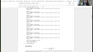
Okay,
so
in
this
next
section
we
will
be
talking
about
the
bird
model
that
has
been
a
landmark
model
in
nlp
when
it
first
came
out.
The
original
publication
took
about
four
days
to
pre-train
the
model
with
a
global
patch
size
of
256,
and
our
team
and
nvidia
tried
to
showcase
optimal
design
techniques
by
scaling
it
up
to
take
only
about
47
minutes,
which
is
a
huge
accomplishment.
B
B
So,
on
a
high
level
to
have
a
successful,
highly
performant
multi-node
system,
you
need
three
things.
The
first
is
the
optimized
software
stack,
so
optimize
system,
design
and
data
center
management.
So
let's
take
a
minute
to
understand
each
of
these
techniques.
So,
first
and
foremost,
we
have
algorithmic
optimizations.
B
This
is
everything
we
can
do
within
a
single
gpu
to
have
a
highly
performing
model
and
we've
already
discussed
some
of
them
using
ncf
as
an
example,
and
then
we
have
the
system
design
so
consider
the
case
of
using
more
than
one
gpu.
We
then
have
to
think
about
the
communication
between
the
gpus
gpu
to
cpu
ratio,
etc,
and
then,
when
we
take
it
a
step
higher
to
multi-node
systems
where
we
need
the
whole
software
stack
to
run
on
a
cluster.
B
B
So
here,
for
example,
they
compared
lars
and
lamb
side
by
side.
On
the
left
hand
side.
You
see
that,
as
we've
discussed
before
on
the
final
step,
we
basically
scale
the
learning
date
with
l2
norm
of
your
base
by
l2
norm
of
your
updates
and
on
the
right
hand,
side.
We
do
something
similar,
but
we
do
it
with
the
first
order,
momentum
and
second
order,
momentum,
mt
and
vt
values.
B
B
So,
for
example,
before
we
do
anything
with
the
gradients,
we
normalized
the
entire
gradients
of
the
model
by
the
l2
norm
of
all
the
gradients
variants,
and
we
saw
that
is
actually
quite
important
to
do
this.
Otherwise
our
model
would
diverge
pretty
quickly
and
and
the
reason
we
think
this
is
necessary
is
because
in
large
batch
settings
where
the
direction
of
your
gradient
is
largely
preserved,
we
don't
want
the
the
gradient
values
to
be
too
high,
and-
and
this
also
alleviates
the
exploding
gradient
problems
and
on
the
right
hand,
side.
B
We
show
the
results
with
bias
correction,
even
though
the
lamp
paper
does
use
bias
correction.
They
mentioned
that
without
bias
correction,
they
were
able
to
converge,
okay
and
but
that's
not
something.
We
noticed.
We
see
that
the
implicit
bias
of
beta,
1
and
beta2
is
actually
pretty
strong
without
bias
correction.
We
see
that
it
diverges
pretty
quickly.
B
B
So
that's
a
kind
of
that
kind
of
wraps
up
our
work
with
optimizer
tricks
today,
so
we
can
move
on
to
the
the
software
stack
section
of
the
optimizations,
so
in
a
regular
back
propagation
for
model
training.
We
see
something
like
this,
where
you
basically
have
your
forward
prop
and
your
update
of
the
weights
and
your
backward
prop,
but,
as
you
can
see
in
the
as
you
can
see,
with
the
green
portion
of
the
timeline,
we're
wasting
a
lot
of
gpu
time.
B
By
simply
waiting
for
this,
I
operations
to
complete
and
we've
noticed
that,
just
by
pipelining,
these
not
pipelining,
sorry
overlapping.
These
I
operations
with
computation.
We
see
a
pretty
good
speed
up
and
a
high
utilization
of
your
gpu.
So
this
is
something
you
can
try
out
as
well
and
the
next
thing
that
we've
noticed
that
really
helps
with
performance
is
fusing
kernels.
So
the
the
thing
about
a
lot
of
the
frameworks
that
we
use
today,
like
pytorch
and
tensorflow,
use
pretty
low
level
operations.
B
But
if
you
can
reduce
all
these
seven
kernels
into
one
kernel,
it
reduces
the
overhead
of
launching
all
of
these
kernels
but
also
improves
the
memory
locality.
So
this
is
a
more
complicated
trick
to
implement
than
the
ones
that
we've
discussed
so
far,
but
we've
seen
that
it
actually
does
help.
So
this
these
are
the
results
we
got
from
students
at
the
vector
institute
that
kind
of
match
the
results
that
we
got
as
well
for
burt.
B
B
We
perform
forward
prop
locally
on
a
particular
gpu,
and
then
we
do
an
nccl
all
reduce
to
collect
all
the
gradients
from
all
of
these
gpus
and
nvidia
implements
an
nccl
communication
library
that
does
this
already
use
efficiently,
but
we
can
see
that
when
you
look
at
the
timeline
of
this
already
use
operation,
you
usually
have
a
forward
prop
a
backward
prop
and
then
an
all
reduce
between
all
of
the
gpus.
Before
you
can
do.
B
So
something
that
you
can
do
to
alleviate
this
is
use
is
overlap
the
already
used
with
backward
propagation.
So,
for
example,
if
you,
if
you're
done
back
propagating
loss
through
the
nth
layer,
you
can
start
all
reducing
it,
as
you
continue
doing,
the
backward
prop
through
n
minus
one
layer,
and
the
good
thing
about
this
is
that
you
don't
have
to
actually
implement
this
yourself.
You
can
simply
use
apex
or
distributed
data
parallel
wrapper
to
your
model.
B
So
all
you
have
to
do
is
say:
model
is
equal
to
ddp
of
model,
and
it's
taken
care
for
you.
So
what
ddp
in
the
in
the
background
does?
Is
it?
Does
the
it
overlaps
the
reductions
with
your
backward
propagation?
So
it
improves
the
utilization
of
your
gpus
and
it
also
does
fp16
reductions
if
you've
activated
amp,
so
instead
of
porting
all
of
these
gradients
to
fp32
and
then
or
reducing
it
and
putting
it
back
to
fp16,
it
directly
does
the
reductions
in
fp16,
which
is
pretty
cool
too.
B
So
gradient
accumulation
is
a
simple
trick
by
which
you
can
do
multiple
forwards
and
backwards
before
you
actually
have
to
all
reduce.
So
in
this
particular
example,
we
are
say
doing
two
forwards
and
two
backwards
before
we
do
an
all
reduce,
and
what
this
essentially
does
is,
let's
say
if
your
batch
size
for
each
forward
prop
is
x
and
by
doing
two
forwards
and
two
backwards
before
you
all
reduce
you
are
emulating
a
batch
size
of
2x.
B
But
again,
all
of
these
this
particular
trick.
Now
that
we
are
emulating
a
higher
batch
size.
We
also
have
to
take
care
that
our
convergence
is
not
affected
by
this
trick,
but
we've
seen
that
this
really
really
helped
us
with
birth.
For
example,
like
I
mentioned
before,
the
batch
size
that
originally
google
was
using
was
256
and
we
scaled
it
up
to
64k
or
96k,
but
the
maximum
batch
size
that
you
can
fit
within
a
gpu
is
only
about
64
for
bird,
because
it's
a
big
model.
B
And
in
this
slide
we
see
with
gradient
accumulation
and
again
on
the
left
side.
We
have
one
machine,
four
gpus
and
on
the
right
side
we
have
four
machines
and
one
gpu.
The
right
side
is
with
a
much
lower
interconnect
speed
and
you
can
see
that
it
scales
quite
well
even
with
low
interconnect,
speeds.
B
So,
coming
to
one
of
the
last
multi
gpu
tricks
that
we've
seen
so
usually
for
training
these
massive
models,
we
have
massive
data
sets.
So,
for
example,
if
you
have
one
input
file
with
all
the
data,
it
is
highly
inefficient
because
each
of
the
gpu
loads,
this
massive
input
file,
which
is
not
efficient.
So
one
of
the
ways
in
which
you
can
optimize
this
is
by
splitting
the
input
files
into
shards
so
that
each
gpu
only
has
to
load
what
it
absolutely
requires.
B
So,
lastly,
to
take
it
one
notch
higher
and
scale
to
multiple
nodes.
Like
we
discussed,
we
need
proper
input,
node
communication,
and
we
should
also
consider
moving
data
close
to
compute
so
that
we
don't
suffer
with
low
interconnect
speeds,
for
example,
moving
the
charts
that
a
machine
needs
closer
to
avoid
data
movement
over
the
network
or
ethernet.
B
B
So
to
conclude,
dl
models
will
continue
to
grow
in
size
and
they
require
massive
scale
out.
That
requires
careful
consideration
on
multiple
aspects.
Some
of
them
are
really
low
effort
as
simple
as
using
an
api,
so
we
should
really
consider
incorporating
them
into
your
stack
to
improve
the
perf,
but
also
your
own
productivity
and
nvidia
does
provide
multi-node
and
deep
learning
solutions,
and
most
of
our
work
is
open
sourced
in
this
particular
github
repository.
B
So
the
first
question
I
see
is
is
ddp
capable
of
launching
multiple
processes
and
multiple
nodes
simultaneously.
In
the
example,
I've
seen,
it
seems
like
you
need
to
spawn
multiple
processes
in
a
single
loop
process.
Yes,
that's
right!
So
gdp
allows
you
to
communicate
between
all
of
these
processes,
but
you
still
need
to
spawn
multiple
processes
from
a
single
root
process.
So,
for
example,
if
you're
launching
a
training
algorithm
on
four
nodes,
you
need
to
launch
your
so
for
pytorch.
B
Ddp,
the
second
question
is:
how
are
results
with
gradient
accumulation
of
two
differ
from
increasing
batch
size
by
a
factor
of
two.
I
think
they
should
be
similar,
so
the
gradient
accumulation
of
two
is
essentially
increasing
the
batch
size
by
a
factor
of
two,
but
they
are
using
used
in
different
scenarios.
B
So,
for
example,
in
your
hardware,
if
you
can
increase
your
batch
size
by
a
factor
of
two,
you
should
totally
do
that,
because
that
results
in
only
one
forward
and
one
backward
prop,
but
gradient
accumulation
is
used
when
you
can't
increase
your
batch
size
by
anymore,
but
still
want
to
optimize
it
by
reducing
the
the
the
lag
that
we
saw.
So
in
that
case,
you
can
try
gradient.
A
B
C
B
Right
so
I
think
algorithmic
limitations
could
just
be
dependent
on
the
model
itself
like,
for
example,
we're
seeing
multiple
optimizations
for
the
model,
let's
say,
for
example,
going
from
bird
to
gpt3.
We
see
massive
improvements
in
the
accuracy,
so
that's
another
limitation
of
the
model
or
algorithm
itself
that
can
be
improved
as
we
go
forward.
Thank
you.
Yeah.
B
Thanks
so
I
see
another
question
we'll
be
using
bert
in
my
company
for
topic:
extraction,
classification
and
customer
sentiment
analysis
using
pytorch.
What
are
the
advantages
disadvantages
of
python
versus
tensorflow
in
case
of
birth
implementation?
So
we
have
at
nvidia
open
source
both
by
torch
and
tensorflow.
For
that
and
they
have
comparable
performance.
B
D
If
I
could
follow
up
on
that,
it
seems
like
nvidia
really
likes
to
work
with
pytorch
like
in
the
mlperf
results.
It's
mostly
pytorch
implementations,
with
the
exception
of
mxnet
for
resnet.
Can
you
comment
on
why
this
is
it's
just
that
nvidia
developers
have
a
preference
for
working
with
pytorch
because
it's
maybe
nicer
to
work
with
or
are
there
actual
like?
Is
it?
Do
you
think
it's
easier
to
get
let's
say
like
compute
performance
gains
out
of
pi
torch
versus
tensorflow
nowadays,.
B
B
I
guess
yeah,
it's
just
a
matter
of
personal
preference,
because
we
don't
really.
We
see
that
a
lot
of
our
customers
have
a
preference
for
tensorflow
or
pytorch,
depending
on
what
they've
been
using
up
until
now,
but
because
for
ml
perf,
specifically,
we
don't
really
have
to
stick
to
one
particular
framework.
It
kind
of
just
depends
on
the
developer,
I
guess-
or
the
team.
A
From
your
experience
like
have
you
actually
seen
cases
where
people
are
trying
to
apply
the
now
golden
rules
for
how
to
scale
things
and
do
a
warm-up
and
use
certain
optimizers
and
all
of
those
things
to
a
completely
different
domain
on
architecture?
And
is
there
something
that
you
can
say
about
that.
B
We
started
off
with
hyperparameters
that
were
used
in
bert,
but,
as
you
might
have
expected,
they
don't
work
off
the
shelf
for
different
data
sets
or
even
different
models.
So
I
think
again
it
comes
back
to
just
doing
the
hyperparameter
search,
but
starting
from
a
point
that
we
know
work
for
similar
models
or
similar
data
sets.
A
If
you,
if
on
this
example,
if
you
get
it
to
conversion
like
to
get
to
a
reasonable
accuracy
on
a
single
gpu,
of
course,
you
might
not
even
pass
through
all
the
data
and
all
that,
but
and
then
you
want
to
scale
it
to
multiple
gpus
which
of
the
hyper
parameters.
Would
the
the
the
model
be
monsters
or
conversions
be
more
sensitive
to
that?
You
think
that
one
needs
to
optimize
those
at
scale
right.
B
Right
so
I
think,
like
we've
discussed
today,
the
hyper
parameters
that
I
would
first
search
for
are
learning
rate
and
warm-up
steps.
Momentum
and
betas
usually
don't
affect
all
that
much.
Maybe
those
are
hyperparameters
that
you
want
to
tune
in
the
end
for
very
small
games
but
yeah.
I
would
start
off
with
learning
great
and
warm-up
steps
too,
with.
B
A
B
A
I
see
so
it
could
be
a
reasonable
strategy.
At
least
you
would
think
too.
If
I'm,
if
I
I've,
designed
my
model
design
everything,
then
I'm
using
adam,
then
the
first
thing
I
should
do
is
at
the
scale
of
a
single
gpu.
I
can
switch
to
lam
optimize
the
parameters
for
lab
and
then
try
to
scale.
You
think
that
that's
a
sound
strategy.
A
C
A
D
I
guess
I
could
ask
another
one,
so
you
know
it's
great.
That
nvidia
is,
you
know
working
on
so
many
different
aspects
of
deep
learning
and
really
kind
of
pushing
on
you
know
the
software,
the
hardware
and
also
the
methods
nvidia,
has
you've
shown
like
great
recommendations
for
things
like
optimizers
like
lars
and
and
lamb
and
nvlan
and
stuff,
like
this
nvidia
kind
of
puts
things
into
you
know
apex
or
deep
learning
examples
repositories
to
make
them
available
for
for
folks
to
use.
I'm
just
sorry.
D
This
is
overly
windy
to
ask
a
simple
question:
what's
nvidia's
strategy
for,
like
is
nvidia
pushing
to
have
things
like
large
lark
optimizer
or
the
new
nv
lam
like
centrally
available
in
the
frameworks
like
pytorch
and
tensorflow?
I
know
like
lark
is
right
now
in
apex
and
lamb
is
in
apex,
but
I
don't
think
heat
land
is
an
apex,
and
it's
only
in
that
repository
right.
B
Right
so
I
think
the
lamp
that
is
in
apex
is
actually
the
the
lamp
version
that
I
mentioned
with
the
tweaks
that
we
made,
I'm
not
sure.
What's
the
process
like
to
go
from
apex
to
pie,
torch
or
tensorflow,
but
I
know
it
with
mixed
precision:
training,
for
example.
It
first
went
into
apex
because
I
think
that's
the
easiest
part
and
then
eventually
it
goes
into
the
framework.
So
I'm
assuming
lamb
will
as
well.
D
D
B
So
a
lot
of
these
tricks
are
a
sort
of
boilerplate.
Do
you
have
any
experience
with
libraries
that
handle
these?
For
you
example
by
dodge
lighting?
Amp
is
a
good
subset,
of
course
yeah.
So
I
think
apex
handles
some
of
these
tricks.
For
you,
a
lot
of
the
optimizers
that
I
spoke
about
today,
as
well
as
amp,
is
on
apex,
as
well
as
the
distributed
data.
Parallel
that
we've
discussed
yeah.
I
think
apex
should
be
good
for
some
of
these
tricks.
A
Maybe
I
can
so
while
we
have
you,
it's
really
good
to
talk
to
someone
who
has
done
a
lot
of
this
in
practice.
So
thank
you
for
answering
all
the
questions,
and
so,
but
maybe
one
more
question
is
about
batch
norm
or
normalization
layers
are
there
I
mean
there
are
multiple
proposals
for
how
to
do
this
in
a
distributed,
setup
right
and
are.
B
A
Confidence
yeah,
I
think
it's
just
like
this
communication
of
stats.
Right,
like
you,
need
to
all
reduce
the
stats
across
the
batch
because
there's
a
different
examples:
dependence,
okay,
a
different
question
is
like
do
you?
Have
you
seen
any
of
this?
Are
you
aware
of
any
of
these
tricks
up
being
applied
to
graph
neural
networks
for
scaling
yeah
like
distributed
training,
large
batch
training
of
graph
neural
networks.
A
Yeah,
okay,
so
it
sounds
good
yeah.
I
think.
Like
a
lot
of
there,
we
have
a
lot
of
applications
that
are
doing
that
and
now
we're
seeing.
Many
of
these
applications
have
extremely
large
amounts
of
of
data
that
you
know.
Training
on
on
8
gpus
on
a
single
node
would
take
days
to
to
do
one
pass
through
the
data
set,
so
those
we
definitely
want
to
explore
how
to
scale
them,
but
conversions
at
scale
is
still
the
main
question
that
we
have
yeah.
Okay,
thank
you.