►
From YouTube: Week 3 - Deep Generative Models - Aditya Grover
Description
More about this lecture: https://dl4sci-school.lbl.gov/aditya-grover
Deep Learning for Science School: https://dl4sci-school.lbl.gov/agenda
A
A
A
So
before
we
start
I'd
like
to
introduce
you
to
aditya
lithia
grover
is
a
final
year
phd
student
at
stanford
university.
His
his
current
research
is
focuses
on
pro
realistic
modeling
for
presentation,
learning
and
reasoning
in
high
dimensions,
and
he
also
focuses
a
lot
in
on
applications
in
science
and
sustainability
such
as
such
as
weather
forecasting
and
electric
batteries.
His
work
has
been
has
appeared
in
several
high
impact
journals
and
has
also
been
deployed
in
production
by
technology
companies.
A
B
However,
it
so
turns
out
that
in
many
cases,
the
raw
data
that
we
collect
for
our
sensors
is
limited
by
the
available
supervision
we
have.
For
example,
this
could
be
labels
for
prediction
and
obtaining
these
kinds
of
labels
as
say
explicit
signals
of
supervision
to
perform.
The
task
at
hand
can
be
a
very
expensive
process.
They
could
be
cost
you
time,
money,
safety
and
so
on
and
forth.
B
Now
there
are
many
ways
in
machine
learning
to
reduce
the
supervision
requirements,
and
this
is
precisely
the
subject
of
a
number
of
fields.
So,
for
instance,
in
classification,
we
can
actively
query
for
labels
of
points
which
are
close
to
the
decision
boundary
between
two
classes
in
reinforcement
learning.
Often
we
have
access
to
only
very
sparse
rewards,
so
we
can
try
to
shape
the
rewards
so
as
to
provide
additional
proxy
signals
for
learning.
B
So
first,
I
want
to
show
that
it
turns
out
that
we
can
do
a
lot
of
amazing
stuff,
even
with
unlabeled
data,
so
we
can
generate
high
resolution
imagery
from
scratch.
All
these
individuals
that
you
see
here
have
been
generated
from
completely
from
scratch,
because
these
are
fictitious
people.
They
don't
exist
in
real
life.
A
B
At
a
very
quick
example
of
how
this
would
work,
so
this
is
in
one
dimensional
example,
so
we
have
sample
access
to
this
ground
to
distribution
which
I've
assumed
is
a
mixture
of
two
gaussians,
and
here
the
first
gaussian
is
three
times
more
likely
than
the
second
one,
so
we
observe
more
samples
from
the
first
mode
as
opposed
to
second
mode.
So
what
we're
going
to
do
is
we'll
first
then
pick
some
model
family
m.
B
B
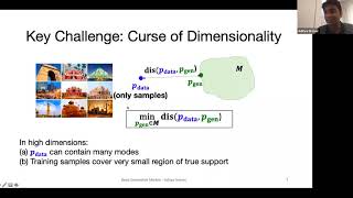
So
often
the
real
world
data
that
we
work
with,
whether
it's
images,
videos
text
or
even
the
different
kinds
of
scientific
data
that
we
have.
It's
hardly
unidimensional
and
the
curse
of
dimensionality
really
makes
things
hard
in
terms
of
this
optimization
problem,
so
intuitively
in
high
dimensions.
We
expect
that
the
data
distribution
will
be
highly
multimodal
and,
moreover,
the
finite
data
set
that
we
have
will
cover
only
a
very
small
region
of
what
we
expect
the
true
support
of
the
data
distribution
to
be
now.
B
These
challenges
have
given
rise
to
a
variety
of
different
generative
models
over
the
last
decade
or
so,
and
what
we're
going
to
see
in
today's
talk
next
is
a
road
map
of
how
we
can
look
at
these
different
families
of
general
models.
What
are
their
pros,
what
are
their
cons
and
what
are
some
of
the
applications
where
these
models
have
been
applied,
particularly
with
regards
to
scientific
discovery?
B
Okay,
so,
let's
start
with
the
first
family
of
generated
models
which
I'm
going
to
call
as
likelihood
based
on
models.
So
we've
seen
a
bit
what
the
why
they
are
called
likelihood
based
it's
to
give
to
spoil
the
fun.
It's
really
the
fact
that
they're
trying
to
maximize
the
likelihood
of
the
data
or
some
approximation
of
it
and
within
this
family.
The
first
example
we're
now
going
to
see
is
the
autoregressive
models.
B
Okay,
so
what
is
an
autoregressive
generator
model?
It's
a
directed,
fully
observed
graphical
model,
so
let's
say
you
have
data
from
which
has
n
dimensions
so
x1
to
xn
are
the
n
dimensions
of
your
data,
and
what
we're
going
to
assume
is
that
every
dimension
here
depends
on
the
previous
dimension.
That
appears
within
some
ordering
that
we
choose.
B
So
here
we
just
choose
the
canonical
ordering
by
the
index,
x1
x2,
so
on
for
x1
and
anytime.
We
have
one
of
these
x's.
It
will
depend
on
all
the
previous
x
dimensions
that
appear
before
it,
okay,
so
the
key
idea
here
is
that
once
we
have
this
graphical
model,
we
can
write
down
its
joint
distribution,
so
the
joint
distribution
of
x,
1,
x,
2
so
on
4
till
x
n.
B
Now
I
mentioned
that
this
is
a
likelihood
based
generative
model,
and
what
this
means
is
that,
when
we
are
trying
to
learn
this
model,
so
by
learning,
we
want
to
find
the
parameters
theta
and
the
objective
we
use
to
find
the
optimal
parameters.
Theta
is
to
maximize
the
log
likelihood
of
our
data
set,
so
the
data
set
that
we
have
so
these
could
be
the
images
of
monuments
that
we
had
a
few
sites
ago.
So
we'll
find
these
parameters
theta,
which
assign
high
probability
to
this
data
set.
B
Now,
if
you
assume
that
the
data
set
is
id,
we
can
write
this
as
a
sum
of
log
probabilities
over
each
of
the
points
in
the
data
set
and
using
the
autoregressive
property.
We
know
that
this
p
theta
of
x
then
can
be
written
in
this
particular
form
where
we
have
factorized
the
joint
distribution
as
the
product
of
conditionals.
B
You
have
a
log
outside,
so
the
product
becomes
log
of
a
product
becomes
the
sum
of
logs,
and
we
have
this
expression
with
us
now.
The
fact
that
we
have
tractable
conditionals-
and
we
see
in
a
few
slides,
which
are
the
various
ways
in
which
we
can
have
these
tractable
conditionals-
allows
us
to
then
evaluate
the
likelihoods
exactly
so
all
the
conditionals
that
we
have
in
that
are
appearing.
This
objective
would
be
evaluated
in
parallel
during
training.
B
Once
we
have
learned
this
model,
so
we
have
found
out
the
best
configuration
of
theta.
What
we're
going
to
then
do
is
at
test
time.
We
want
to
use
this
model
to
generate
more
data
or
another
word
sample,
and
in
order
to
do
so,
the
fact
that
it's
a
directed
model
helps
so
what
we're
going
to
do
is
we're
going
to
sample
one
variable
at
a
time
so
first
we'll
sample
x1.
B
So
you
can
think
of
x1
as
the
first
pixel
of
an
image,
then
we
sample
x2
condition
on
x1,
so
we
sample
the
second
pixel.
That's
conditioned
on
the
first
pixel
of
an
image
and
we'll
keep
doing
this
so
on
and
forth
until
we
have
completed
our
image
and
that
x1
through
xn
will
then
be
our
full
image
composed
of
the
various
pixels
that
we
sampled
okay.
So
this
is
a
tutorial
about
deep
general
models.
So
where
is
the
deep
aspect
of
this?
B
So
the
earliest
variants
of
autoregressive
gender
models
used
factorizations,
which
were
linear,
so
they
went
by
the
name
of
fully
visible
sigmoid
belief
networks.
Over
the
years
people
thought
about
using
neural
networks
so
in
need.
There
was
a
one
hidden
layer,
neural
network
that
was
used
to
parameterize
these
conditionals,
and
this
was
extended
to
having
multi-layer
neural
networks
in
made
as
well
linear
or
multi-layer
perceptron
base.
B
Parameterizations
are
not
the
only
ones
so
for
a
lot
of
high
dimensional
data,
we
can
use
other
deep
architectures,
which
have
other
kinds
of
invariances,
for
example,
for
a
textual
data.
It's
often
useful
to
use
an
rn
based
parameterization,
so,
for
instance,
if
you
want
to
be
able
to
generate
text.
So
what
we're
going
to
do
is
in
this
example,
we
can
see
we
have
a
string
h-e-l-l,
so
we're
effectively
trying
to
train
the
model
by
feeding
it,
the
string
hello.
B
So
what
we
can
have
is
he'll
have
an
rnn
that
looks
at
h
and
then
tries
to
predict
what
is
the
next
character
going
to
be
so
in
this
particular
example,
we
are
assuming
a
simple
vocabulary
where
it
can
just
be
h.
E
l
or
o,
and
the
model
is
going
to
then
try
to
assign
probabilities
for
each
of
these
different
characters
and
by
training
it.
We
are
hoping
that
it
assigns
higher
probability
to
strings
that
are
more
likely
to
appear
in
our
training
dataset.
B
So
this
is
not
just
been
used
for
text,
so
variants
of
it
have
also
been
used
for
images,
so
an
image
we
can
think
of
trying
to
generate
a
pixel
x.
I
conditioned
on
everything
that
appears
before
it
in
a
raster
scan
order
and
again
this
conditional
can
be
parameterized
with
a
recurrent
neural
network
there
for
other
for
data
types.
Many
data
types
also
cnn
based
parameterizations
have
been
explored.
B
So
pixel
cnn
is
a
really
good
example,
where
the
convolutions
that
are
used
in
normal
cnn
are
must,
and
the
masking
is
done
so
that
we
preserve
the
autoregressive
property.
So
if
we
want
to
predict
pixel
here,
we
only
want
to
be
looking
at
pixels
in
the
nearby
region,
but
nothing
that
comes
after
this
pixel,
and
for
that
purpose
we
need
to
mask
the
convolution
the
convolutional
neural
networks,
so
wavenet
is
another
example.
B
That's
been
used
for
audio,
so
in
audio
often
we
want
to
capture
very
long
range
sequences,
so
here
we
use
1d,
convolutions
and
what's
interesting
about
these
1d
convolutions
that
they
are
dilated.
So
if
you
look
at
every
hidden
layer,
we
are
successfully
skipping
more
and
more
units
that
come
before.
So
in
the
first
hidden
layer
we
have
a
dilation
factor
of
one,
which
means
that
if
we
want
to
be
able
to
predict
an
output
for
the
next
layer,
we
will
be
skipping
one
of
the
hidden
activation
that
come
before
it
in
the
sequence.
B
So
all
those
models
about
gpd
are
in
fact,
auto
regressive
models
and
the
key
innovation
that
has
led
to
such
impressive
results
in
those
style
of
models
is
the
use
of
a
transformer
based
architecture
for
parameterizing,
these
conditionals
all
right.
So
this
was
all
I
wanted
to
talk
about
autoregressive
models,
which
is
our
first
kind
of
likelihood
general
model.
B
Okay,
seeing
none
so,
let's
move
on
so
let's
go
to
rational
encoders,
okay,
so
now
there
is
no
encoders,
so
we'll
again
think
of
them
first
as
a
graphical
model,
and
then
we'll
think
about
how
that
graphical
model
can
be
used
for
learning
and
inference
okay,
so
these
models
are
again
directed
latent
variable
models.
So
the
new
thing
that
we
have
from
before
is
this
latent
variable
z.
So
we
didn't
have
a
concept
of
latent
variables
previously,
when
we
were
discussing
other
regression
models.
B
B
Given
this
model,
which
is
goes
from
z
to
x,
we
are
again
interested
in
a
likelihood
based
objective,
so
we
saw
previously
that
in
a
likelihood
based
objective,
our
goal
is
to
maximize
the
log
likelihood
of
the
observed
data
set.
We
only
observe
x's.
So
what
we're
really
interested
in
is
maximizing
the
marginal
log
likelihood
of
the
data
set
where
marginalization
here
means
summing
out
all
the
things
we
do
not
observe.
So
we
do
not
observe
z,
so
we
want
to
then
just
marginalize
it
out.
B
While
we
are
trying
to
learn
the
parameters
theta
for
this
model.
Okay,
now,
as
we
see
that
this
is
actually
going
to
be
a
hard
problem,
and
which
is
why
I
have
this
dotted
arrow
here,
which
is
going
to
be
making
this
problem
much
more
tractable?
Okay,
so
let's
not
pay
too
much
attention
to
this,
but
keep
it
at
the
back
of
our
minds
that
you're
going
to
have
an
inference
network
queue
which
is
going
to
be
helping
us
optimize.
This
objective?
B
B
So
here
my
you're,
assuming
z,
is
continuous,
so
we'll
be
doing
an
integration
here
now,
if
looking
at
this
problem,
one
challenge
is
that,
even
though
each
of
these
joint
distributions
could
be
tractable,
so
we
could
evaluate
it
for
a
single
z.
Then
we
have
a
high
dimensional
or
or
a
continuous
space
for
z.
Then
it
might
be
very
hard
to
be
integrating
it
out,
analytically.
B
So
this
challenge,
what
it
necessitates
is
that
what
we're
going
to
do
is
we
look
at
a
particular
distribution,
which
is
we
call
the
posterior
distribution,
so
this
posterior
distribution
is
can
be
extracted
from
the
joint.
So
it's
the
distribution
or
z
conditioned
on
x
and
the
key
idea
that
we'll
exploit
is
that
this
distribution,
if
we
approximate
it
with
something
analytical
something
simple
like
q
and
q,
is
something
which
we'll
choose
on
our
own,
then
this
objective
actually
becomes
tractable
to
optimize.
B
So,
let's
look
at
how
this
works
out
in
more
detail,
so
we
said
that
marginalizing
out
this
joint
distribution
is
going
to
be
intractable.
There
are
lots
of
z's
out
here,
so
we'll
do
a
a
simple
math
to
derive
a
tractable
objective.
So
what
we
do
here
is
we
multiply
both
the
numerator
and
denominator
by
this
distribution,
which
we
are
calling
as
the
approximate
posterior,
cue,
okay,
so
q,
you
can
think
of
it.
It
takes
an
x
and
then
it
maps
it
to
a
distribution
over
the
latent
itself.
B
Now,
by
genesis
inequality,
we
can
then
write
an
inequality
which
will
basically
push
out
this
approximate
distribution.
Q
outside
the
log,
so
from
jensen's
equality,
log
of
an
expectation
exceeds
or
is
equal
to
the
expectation
of
the
log
of
the
term
itself.
Okay,
so
just
by
pushing
out
q
outside,
we
are
left
with
this
objective.
B
B
So
this
objective
is
what
we're
going
to
be
calling
as
album
and
what
it
stands
for
is
the
evidence
lower
bound
of
our
data.
So
we
had
a
data
point
x
and
for
that
data
point
x
we
were
able
to
use
p
and
q
to
write
an
objective
which
looks
like
an
expectation
now.
One
question
to
ponder
over
is
that,
when
does
when?
Is
this
inequality
tight?
B
B
It's
going
to
be
constant,
but
what
we're
trying
to
do
is
then
we're
trying
to
optimize
for
the
parameters
phi
such
that
the
resulting
lower
bound.
The
elbow
here
becomes
tighter
and
tighter,
hopefully
getting
close
to
the
true
log,
marginal
likelihood
estimate
and
what
will
control
the
quality
of
our
approximation
is.
How
small
is
the
kl
gap
between
our
evidence
lower
bound
and
the
log
marginal
likelihood.
B
So
this
gap
here
is
the
kl
divergence
between
q
of
z,
given
x
and
b
theta
of
z
given
x,
so
in
practice,
both
theta
and
p,
are
something
we
do
not
know,
and
this
gives
us
an
autoencoder
perspective
of
thinking
about
this
model.
So
here
is
again
our
learning
objective,
which
is
an
expectation
of
the
log
of
this
quantity
with
respect
to
the
approximate
posterior
q
and
we
can
decompose
this
term.
B
Now
we
should
think
of
this
term
as
exactly
the
objective
of
an
auto
encoder.
So
in
an
auto
encoder
you
feed
in
an
input
x
and
you
pass
it
through
an
encoding
phase
and
after
an
encoding
phase,
which
we'll
think
of
as
parameterizing
the
distribution
queue,
we
get
a
distribution
over
latents
the
parameters
mu.
B
B
A
B
Innovation,
auto
encoder,
the
mapping
from
x
to
z,
has
some
stochastic,
because
z
is
some
random
variable
that
we
do
not
know.
So
what
we're
really
learning
is
the
parameters
of
the
distribution
over
c,
that's
the
first
term,
the
second
term,
which
is
the
scale
term
hanging
around
there.
So
it's
trying
to
bring
the
approximate
posterior
cures
given
x,
close
to
some
prior
distribution
over
c,
okay,
so
the
prior
distribution
over
z,
something
that
we
can
choose
or
we
can
also
learn.
B
B
So
that's
the
auto
encoder
perspective
of
how
these
models
are
typically
learned.
The
architecture
looks
very
much
like
a
standard,
auto
encoder,
but
the
objective
that
we
have
here
has
some
additional
nuances.
So
the
z
here
is
stochastic
and
we
have
an
additional
term
here,
which
accounts
for
the
kl
divergence
between
our
approximate
posterior
and
the
prior
that
we
have
here.
B
Okay,
so
we
discussed
how
we
can
learn
by
maximizing
this
evidence
overbound,
if
our,
if
we
can,
if
our
encoder
is
very,
very
powerful
and
we
recover
the
true
posterior.
This
is
our
bound
is
tight,
but
even
if,
in
general
that
doesn't
happen
to
be
the
case,
we
can
still
hope
to
get
close
to
the
true
marginal
log
likelihood
of
the
data.
B
It's
a
directed
model.
So
again
we
can
do
ansys
to
the
sampling.
When
we
are
sampling,
we
throw
away
the
encoder.
All
the
work
is
the
decoder,
so
we
sample
z
from
some
prior
distribution
and
then
x
can
be
sampled
from
the
conditional
of
a
distribution
of
x,
given
z,
which
is
parameterized
by
the
decoder.
B
Why
did
we
introduce
later
variables
in
the
first
place?
One
useful
thing
about
latent
variable
models,
especially
in
va,
is
that
we
can
use
the
encoder
to
then
directly
learn
some
representation
of
our
input
point
x.
So
if
you
want
to
learn
a
representation
for
let's
say
for
clustering
for
visualization
or
for
some
downstream
tasks,
then
all
we
have
to
do.
Is
we
take
any
data
point
x
and
we
pass
it
through?
B
Our
encoder
and
then
we
look
at
what's
the
latent
distribution
that
we
learn
over
z
and
that
latent
distribution
is
going
to
contain
some
mean
parameters
and
some
standard
deviation.
If
we
assume
the
distribution
to
be
a
gaussian,
and
these
parameters
themselves
then
become
a
representation
for
the
input
x
that
we
can
use
for
some
downstream
tasks.
B
Okay,
so
these
models
have
they've
been
a
lot
of
progress
over
the
years.
This
is
a
work
from
just
last
month,
where
a
hierarchical
version
of
this,
where
we
have
multiple
layers
of
stochasticity,
so
not
just
one
z,
but
there
are
also
many
many
layers
of
stochasticity
within
the
model.
If
we
apply,
if
you
use
that
model
and
then
use
some
other
training
tricks,
we
can
obtain
very
high
resolution
imagery
once
we
have
printed
these
models.
B
Okay,
so
I
also
want
to
give
in
just
one
picture:
what
are
some
promising
directions
for
extending
these
models
in
case?
Some
of
you
are
interested
so
essentially
the
name
of
the
game
for
variational
order.
Encoders
is
to
approximate
this
posterior
distribution,
p
theta
of
z,
given
x,
with
some
tractable
distribution,
q
of
phi
of
z.
B
So
we
start
with
some
initial
start
state
for
the
encoder
parameters
fee,
and
then
we
are
trying
to
update
both
the
encoder
parameters
from
v,
as
well
as
the
decoder
parameters
theta,
so
that
they
get
to
some
optimal
theta,
star
and
v
star,
and
this
in
general
can
be
a
highly
non-convex,
optimization
problem.
So
thinking
about
what
a
good
optimization
technique
specifically
for
this
objective
is
one
way
of
one
way
of
making
these
models
better.
B
B
Finally,
why
should
we
compare
these
distributions
q
and
p
theta
just
by
the
kl
versions,
so
there's
also
been
exciting
works
which
look
at
how
we
can
consider
alternate
ways
of
comparing
these
distributions
using
divergences,
which
are
other
than
the
k.
Otherwise,
for
instance,
the
vast
string,
divergence,
the
vastus
team
distance
and
the
maximum
needs
mean
discrepancy
and
all
these
various
families
of
probabilistic
divergences
and
distances
that
people
have
come
up
in
other
contexts
as
well.
B
A
B
That's
a
great
question,
so
the
question
about
so
general
models
here
what
we
are
so
it's.
The
first
thing
is
like:
how
do
we
define
extrapolation
so
if
you're
thinking
about
extrapolation
in
the
context
of
data
generation,
so
maybe
one
notion
of
extrapolation
could
be
that?
Oh,
if
I
see
a
model,
that's
trained
on,
let's
say
blue
circles
and
red
triangles:
do
we
expect
the
model
to
generate
blue
triangles?
That
would
be
some
form
of
maybe
extrapolation
in
some
sense
that
never
saw
that
during
training.
B
But
it's
trying
to
then
generate
something.
That's
new
and
the
short
answer
to
that
is.
It
depends
on
what
inductive
biases
are
based
baked
into
the
model.
So
if
the
inductive
biases,
for
instance,
is
invariant
to
the
combinations
of
colors
and,
let's
say
shapes
in
this
particular
toy
example
that
I
made
up
then
sure
it's
possible
that
it
disentangles
those
factors
in
the
training
set
and
even
during
test
time,
then
it's
able
to
make
up
these
new
combinations
of
shapes
and
colors
that
never
saw
during
training
so
yeah.
B
B
B
Yes,
so
I,
as
I
said,
there
are
two
differences,
and
this
slide
illustrates
them
best.
So
here,
if
let's,
let's
see
what
a
regular
encoder
would
do,
it
would
take
some
input.
It
would
pass
it
through
an
encoder
and
the
output
of
the
encoder
will
be
some
compressed
representation
of
the
input
x
and
it
will
use
that
compressed
representation
directly
to
then
reconstruct
the
input
during
the
decoding
phase.
B
So
that's
the
one
way
in
which
the
forward
pass
through
the
vational,
auto
encoder
differs
from
a
regular,
auto
encoder
and
then
another
difference
which
comes
about
when
we're
actually
trying
to
learn
this
model
via
back
propagation.
Is
that
the
objective
not
just
contains
a
reconstruction
error
term,
which
also
occurs
in
a
regular,
auto
encoder,
but
there's
an
additional
term
which
comes
about
from
the
elbow
objective,
which
tries
to
regularize
the
approximate
posterior
q
of
z
given
x,
which
is
what
the
encoder
learns
with
some
prior
distribution
over
c.
B
So
this
is
an
additional
piece
of
the
puzzle
that
we
have
to
pick.
So
we
have
to
pick
some
prior
over
how
we
want
our
latent
codes
to
be
so
if
we
believe
the
latent
code
should
look
like
a
gaussian,
we
can
set
this
to
be
a
gaussian,
and
this
term
would
ensure
that
if
we
maximize
the
elbow
we'll
have
to
minimize
the
scale
divergence
so
we'll
try
to
regularize
our
encoder
outputs
to
look
close
to
that
of
a
gaussian.
A
We
have
many
many
more
questions,
so
maybe
we
can
take
one
or
two
more
and
then
see
how
the
other
one
is
so
other
regressive
models
try
to
build
relationship
from
earlier
data
to
later
data.
This
seems
like
the
model
will
depend
on
what
you
decided
earlier,
like
in
the
case
of
image.
Pixels
is
the
direction
chosen
in
training
or
do
people
build
ensemble
of
models
using
different
directions.
B
B
So
here
we
have
to
pick
an
ordering
of
the
dimensions
of
x
so
from
x1
to
x2
so
on
to
xn,
who
picks
that
ordering
now
that
ordering
is
something
that
we
decide
beforehand.
So
in
the
case
of
let's
say
images,
the
ordering
is
typically
raster
scan.
So
you
start
from
the
first
pixel
on
the
top
left
and
then
you
go
within
a
row
and
then
you
go
on
to
the
next
two
and
so
on
forth,
and
that
way
you
specify
an
ordering.
There
have
been
works
which
are
order
agnostic.
B
B
So
the
benefits
of
autoregressive
models
are
that
these
are
actually
very,
very
expressive.
So
if
the
conditionals
could
represent
any
distribution,
then
the
overall
joint
probability
could
also
approximately
distribution.
So
this
is
just
by
the
chain
rule.
So
by
the
chain
rule
we
can
write
the
joint
probability
of
the
product
of
these
conditionals.
So
if
we
make
these
theta
or
the
neural
networks
very
very
expressive,
we
can
actually
represent
any
distribution
over
x.
B
B
B
B
So
there
is
a
latent
variable,
z
and
then
there's
some
observables
x,
but
we
makes
one
change,
which
is
that
we
will
think
of
z
mapping
to
x
in
a
deterministic
and
invertible
manner.
Okay,
so,
instead
of
having
some
arbitrary
mapping
between
z
and
x,
we'll
say
that
z
and
x
will
have
the
same
dimensionality,
so
both
will
be
n,
dimensional
objects
and
the
way
we
can
transform
a
sample
from
the
prior
distribution
over
z
to
a
sample
of
x
will
be
via
deterministic
and
invertible
mapping,
which
I'm
denoting
as
f
theta.
B
So
because
it's
invertible
by
design,
if
you
want
to
get
z
once
we
have
an
x,
we
just
use
the
inverse
of
f
to
get
back
our
c.
So
let's
look
at
an
example.
So,
for
example,
we
could
have
z
the
distribution
over
z
being
denoted
uniformly
over
the
square,
and
now,
if
we
apply
a
transformation
to
it
in
this
case,
the
transformation
is
basically
multiplying
by
a
2
cross,
2
matrix
with
entries
a
b
c
and
d.
B
So
if
we
want
to
find
out
what
is
the
probability
of
some
data
point
x
in
the
space
defined
by
this
random
variable
big
x,
we
can
write
this
probability
density
as
the
product
of
the
prior
density
over
z
times
the
absolute
value
of
the
determinant
of
the
jacobian
of
the
inverse
of
f
with
respect
to
x.
Okay.
B
So
this
is
the
additional
term
that
controls
how
much
do
the
volumes
change
as
we
move
from
the
space
of
z
to
the
space
of
x
so
like
in
this
case,
if
we
go
from
the
space
of
z
to
space
of
x,
you
can
see
that
there's
a
change
in
volume.
The
square
here
has
a
different
volume
than
the
parallelogram
here,
and
this
jacobian
term
essentially
controls
that
change
in
volume.
B
B
This
is
the
jacobian
term,
and
here
we're
looking
at
the
absolute
value
of
the
determinant
of
the
jacobian,
which
quantifies
precisely.
What's
the
per
unit
change
in
volume
when
we
go
from
z
to
x
by
the
mapping
f
here
now,
that's
the
so
one
thing
to
notice
about
this
expression
is
that
this
density
is
already
normalized.
So
if
z
was
normalized,
we
can
pick
any
invertible
transformation
f
and
the
distribution
that
we
get
for
x
is
going
to
be
a
normalized
distribution.
B
So
it's
going
to
integrate
to
one
it's
going
to
be
positive,
so
we
get
tractability
for
free,
which
was
not
the
case
when
we
had
various,
not
encoders,
so
remember,
invasion,
auto
encoders
we
had
it
was
intractable
to
get
the
marginal
likelihood
over
x.
So
what
we
did
was
we
considered
an
evidence
lower
bound
to
the
margin
log
likelihood,
but
here
by
constraining
f
to
be
invertible,
we
can
just
apply
the
change
of
variables
formula
and
get
a
normalized
distribution
for
free
now.
B
The
other
thing
that
you
see
in
this
terminology
is
that
it's
called
the
flow
and
the
reason
why
it's
called
the
flow
is
because
these
invertible
transformations
f
theta
can
actually
be
composed
with
each
other.
So
if
you
apply,
if
you
compose
invertible
transformations,
the
result
is
another
invertible
transformation.
B
So
what
do
these
transformations?
Do?
We
said
that
geometrically
they
seem
to
be
shrinking
or
shearing
or
expanding
the
probability
densities
in
a
geometric
sense.
So
here's
an
example
where
a
bunch
of
these
invertible
transformations
were
applied
and
what
they
did
was
if
we
start
with
m
equals
0,
which
means
we
have
no
transformation,
so
we're
just
looking
at
the
prior
density
of
z,
zero.
That
was
gaussian
distributions.
B
But
as
we
successfully
applied
more
of
these
transformations,
we
can
see
that
the
shape
of
the
distribution
starts
changing.
So
these
contours
start
reflecting
more
complex
patterns
which
could
be
a
better
approximation
to
the
data
at
hand
for
which
this
model
was
trained.
So
with
just
10
transformations.
We
have
seen
that
we
can
learn
very
complex
distributions
using
these
models.
B
Okay,
so
how
do
we
learn
the
parameters
of
these
transformations
that
we
apply?
Well,
we
have
the
log
marginal
likelihood
in
closed
forms,
so
we
can
just
use
the
maximum
likelihood
estimation
objective
without
having
to
do
with
variational
inference.
So
this
is
similar
to
how
we
were
exactly
optimizing
for
the
log
likelihood
in
the
case
of
an
autoregressive
model,
and
we
can
see
that
by
using
change
available's
formula,
we
can
get
a
handle
on
the
exact
likelihoods.
B
Now
this
was
the
learning
aspect
at
test
time.
We
want
to
do
inference
with
this
model,
and
one
task
we've
been
considering
is
that
let's
say
we
want
to
sample
from
this
model,
so
it's
a
direct
latent
variable
model,
so
we
know
we
can
use
answers
to
the
sampling,
so
we
sample
z
from
some
prior
distribution
over
z
and
then
to
get
the
actual
sample
x.
We
passed
it
through
the
invertible
transformation
f.
B
B
Okay.
So
these
models
have
also
demonstrated
a
lot
of
success,
and
here
is
one
of
these
models
glow,
so
the
mean
area
of
research
within
normalizing.
The
models
is:
how
do
we
specify
these
invertible
transformations
f
and
glow
here
again
used
a
variant
of
1d
convolutions,
where
they
were
able
to
obtain
samples
which
can
do
very
well
at
interpolating
across
different
latent
attributes?
B
For
example,
here
are
the
two
authors
of
this
paper,
so
this
is
the
kingma
who
was
also
one
of
the
co-inventors
of
ease
and
here's
praful
dharwal,
who
was
also
on
this
paper
and
now,
if
we
see
how
running
this
model,
we
can
interpolate
across
the
different
latent
attributes.
So
for
the
same
person
we
can
vary
attributes
such
as
the
presence
of
a
beard,
the
hair,
color
and
so
on
and
forth.
B
I
think
okay,
so
we
haven't,
talked
about
adversarial
learning,
but
we'll
do
that
next,
but
an
adversarial,
auto
encoder,
essentially
optimizes
for
a
different
divergence
from
kl
divergence
in
the
latent
space.
So,
like
I
said
one
of
the
areas
of
research
within
vaes,
let
me
go
back
to
this.
Slide
is
thinking
about
whether
kale
divergence
is
the
right
notion
of
divergence
between
our
approximate
posterior
q
and
our
true
posterior
p,
and
in
an
adversarial,
auto
encoder.
B
B
B
So
when
I
talk
about
gans
or
teach
about
it,
they're
like
many
many
different
perspectives
with
which
you
can
think
about
gans.
The
perspective
that
I
like
to
think
best
summarizes
is
gans.
Is
it's
a
likelihood
free
mod,
so
all
the
models
that
we
saw
so
far,
whether
it
was
autoregressive
models
or
vaes
or
whether
it
was
normalizing
from
models?
They
were
trying
to
approximate
the
log
likelihood
of
the
data,
either
ex
or
in
the
case
of
autoregressive
models
and
flow
models.
That
was
exact.
B
B
We
can
also
think
of
models
and
training
objectives
which
do
not
require
the
likelihood
okay.
So,
let's,
if
you
see
this
picture
this
discrepancy,
if
we
have
a
likelihood
model,
this
discrepancy
is
essentially
the
kl
divergence
and
now
what
we're
going
to
see
is
in
gans
a
different
way
of
specifying
this
discrepancy.
B
So
how
it
looks
like
is
that
again,
we
want
to
find
some
generative
model
between
within
small
family
m,
but
the
way
we
specify
the
differences
between
the
general
model
and
the
true
data
distribution
is
by
looking
at
samples
from
the
data
distribution,
p
data
and
the
generative
model
pj,
and
for
these
samples
we'll
then
compare
their
expectations
of
some
function.
F,
so
f
is
some
function,
so
you
can
think
of.
It
might
be,
let's
say
a
mean
function,
so
you
look
at
samples
from
the
data
distribution.
You
look
at
samples
from
the
general
model.
B
We
are
able
to
then
find
the
best
general
model.
So
this
is
our
notion
of
how
we
compare
a
data
distribution
and
a
general
model.
We
specify
some
family
of
functions
f
and
then
we
find
the
member
of
this
family
f,
which
maximizes
the
difference
in
expectations
with
respect
to
the
data
distribution
and
the
general
model.
B
Now
different
choices
of
f
lead
to
popular
discrepancy,
metrics
that
have
existed
for
many
many
decades
and
years
and
have
been
used
in
probability
theory
for
a
very
long
time.
For
instance,
if
we
pick
f
to
be
the
class
of
bounded
r
khs's
that
occur
within
the
kernel,
literature,
what
we
get
is
a
maximum
mean
discrepancy
metric
and
similarly,
by
choosing
different
s,
we
can
get
the
total
relation
difference
distance
and
we
can
get
the
versus
time
distance
as
well.
B
Okay.
So
this
is
the
learning
objective,
so
it's
I
call
it
the
two
sample
testing,
because
it's
comparing
two
sets
of
samples,
one
from
the
data
distribution,
one
from
the
general
model
notice
that
here
when
we
specify
the
subjective
we
never
made
use
of
the
likelihood
here.
So
we
never
asked
while
trying
to
evaluate
this
objective,
what
is
p
gen
of
x,
which
would
have
been
the
likelihood.
B
B
B
B
So
real
examples
are
those
that
come
from
the
data
distribution
and
the
fake
ones
are
what
we
might
get
from
the
generator
here.
This
does
not
really
look
like
a
monument,
but
this
generator
is
trying
to
fool
the
critic
into
making.
It
believe
that
it
is
okay,
so
now
during
learning,
both
the
generator
and
the
critic
are
updated.
Alternatively,
so
here
is
an
example
from
the
original
gan
paper,
so
we
have
some
z
here
which
is
pictorially
depicted
on
this
1d
line
and
it
maps
to
some
x's
here.
B
B
Now
so
this
is
how
learning
works.
We
can
also
think
about
inference.
So
I,
like,
I
said
the
way
we
learn.
These
models
is
by
a
likelihood
free
objective.
So
if
we
really
care
about
the
likelihoods,
we
might
actually
not
have
access
to
them
in
a
tractable
manner.
Are
some
exceptions
we
can
consider.
So
if
you
do
consider
the
class
of
invertible
models
like
within
flow,
in
that
case,
we
can
also
evaluate
the
likelihoods
there's.
B
B
Okay,
so
over
the
years
gans
have
made
rapid
strides
in
sample
quality.
So
around
the
time
when
I
started
my
phd,
the
original
gantt
paper
came
about
in
2014
and
every
year
since
then,
it's
been
higher
resolution
harder
to
detect
whether
each
of
these
samples
are
actually
real,
and
one
might
actually
think
that
oh
have
these
models
really
passed.
B
Now
these
models
are
used
for
so
many
different
tasks.
This
is
one
really
impressive
task
for
which
these
models
were
applied.
So
here
what
was
done
was
we
have
two
sets
of
samples,
so
we
might
have
the
paintings
on
my
name
and
we
might
have
the
photographs
that
we
might
have
clicked
ourselves
from
on
our
camera,
and
what
we're
trying
to
do
is
we're
trying
to
learn
mappings
from
one
set
of
images
to
another,
so
we
can
think
about.
B
So
again,
another
example
is,
let's
say
we
have
a
data
set
of
zebras
and
the
data
set
of
horses,
and
we
want
to
think
about
okay.
How
would
in
the
same
scene,
if
we
had
these
zebras
if
they
were
actually
horses?
How
would
these
look
like
and
again
we
can
use
this
translation.
We
can
also
do
it
in
the
reverse
direction,
so
you
might
have
a
horse
and
we
want
to
see
oh
what,
if
this
horse
is
actually
a
zebra
in
the
same
environment
and
again,
we
can
use
a
conditional
gun
for
these
translations.
B
Okay.
So
this
finishes
what
I
wanted
to
say
about
generative
adversarial
networks
and
I'm
gonna
spend
maybe
five
minutes
or
so
on.
Talking
about
the
different
kinds
of
scientific
applications
which
might
be
of
interest
a
lot
of
people
attending
this
virtual
seminar,
as
well
as
give
some
concluding
thoughts
about
what
exciting
research
directions,
both
from
an
algorithmic
and
from
a
practical
perspective,
with
these
models
before
I
do
those
are
there
any
questions
about
gans
that
I
can
answer.
A
B
Good
questions:
the
question
is:
let's
go
back
here
so
here
we
said
we
have
to
assume
something
for
the
prior
distribution,
and
I
said
that,
oh,
we
can
let
it
be
a
standard,
gaussian
standard,
normal
distribution.
What,
if
that's,
not
a
good
distribution?
Indeed,
there
is
a
lot
of
works
and
I
can
link
them
offline
where
learning
the
prior
distribution,
as
opposed
to
keeping
it
fixed
to
be
a
gaussian,
can
actually
give
a
lot
of
improvements
in
the
performance
of
these
models.
B
So
there
have
been
works
in
fact,
which
often
think
of
this
prior
as
being
an
auto
regression
model
itself.
So,
instead
of
having
standard
gaussian
distributions,
which
is
not
assuming
any
correlational
structure
amongst
the
dimensions
of
z,
you
can
actually
enforce
them
to
have
an
autoregressive
dependency,
and
that
does
very
very
well
for
some
advanced
variants
of
these
models.
B
Okay,
another
another
great
question,
and
this
is
one
of
the
pressing
research
directions
within
the
gans,
which
is
that
in
practice,
this
minimax
optimization
problem
is
very
hard
to
solve,
even
for
very
simple
choices
of
the
model
family
that
we
pick
for
the
generator
and
discriminator.
This
can
be
very
hard,
and
when
that
is
the
case,
then
doing
this
alternating
mini
max
optimization
problem
might
often
give
you
make
you
land
at
points
where
there
is.
B
The
generator
is
just
producing,
essentially
garbage
output,
because
the
optimization
has
failed,
the
discriminator
could
be
very,
very
powerful
and
the
gradients
might
not
be
back
propagating
to
the
generator
in
a
suitable
manner.
So
that's
often
that's
called
as
mode
collapse.
So,
if
you
might,
some
of
you
might
have
heard
of
this.
So
what
happens
in
mode
collapses?
B
So
that's
a
persistent
problem
with
cans
and
an
active
area
of
research
about
what
are
different,
optimization
techniques
that
can
be
used
other
than
the
vanilla
gradient
descent
in
an
alternating
fashion
that
people
use.
So
if
I
have
to
just
pick
one
of
them,
so
another
thing
that
helps
is
in
optimization
is
thinking
about
what
this
function.
Class
f
is
so,
for
instance,
it's
been
shown
in
recent
work
that
if
f,
corresponds
to
what
would
lead
this
objective
to
correspond
to
the
versus
time
distance.
A
B
Yeah
so,
like
I
mentioned
here
that
empirically
people
have
seen
that
when
you
use
the
vasos
time
distance,
it
has
better
geometries
it.
It
accounts
for
the
geometry,
unlike
a
lot
of
these
divergences,
scale,
differences
which
are
invariant
reparameterizations
and
that
in
a
sense,
stabilizes
optimization
and
gives
better
results
in
practice.
A
B
B
So
what
is
the
motor
mode
is
any
region
of
the
distribution
which
has
high
probability
mass
so,
for
instance,
it's
a
mixture
of
two
gaussian,
so
there
are
two
modes
of
the
distribution,
but
in
this
case
we
know
that
they're
two
modes,
because
we
cheated
in
this
toy
example,
because
we
knew
what
the
data
distribution
was
now
in
practice.
If
I
see
a
real
data
distribution
like
let's
say,
I
see
this
images
of
monuments,
then
it's
hard
for
me
to
say
how
many
modes
are
there
in
such
high
dimensional
distributions.
B
So
you
see
how
well
it
covers
those
following
modes
in
a
mixture
of
body
gaussians,
and
that
will
give
you
some
sense
of
how
much
mode
covering
behavior
that
exists
in
that
model
for
real
distributions
you
wouldn't
for
real.
You
would
have
to
make
some
sort
of
approximations
of
what
your
mode
could
correspond
to.
For
example,
if
you
have
label
data
sets,
so
let's
say:
if
you
had
labels,
let's
say
imagenet
or
in
c4
or
these
kinds
of
data
sets.
B
B
B
So
I'm
just
going
to
read
out
some
of
these
titles,
so,
for
example,
here
is.
The
here
is
an
example
where
the
first
paper
here
physics
aware
deep
general
models
for
creating
synthetic
microstructures.
So
what
these
models
did
was
they
infused
some
physical
structure
within
the
genital
model
and
they
used
it
for
materials
discovery?
In
this
case
those
materials
corresponded
to
microstructures
the
second
work.
B
This
is
a
very
prominent
work,
so
this
was
one
of
the
first
works
which
showed
how
you
can
do,
let's
say,
drug
discovery
using
these
models.
So
what
happened
in
these
models?
We
used
a
rational,
auto
encoding
style
of
framework,
so
in
the
latent
space
they
essentially
perform
bayesian,
optimization
and
anytime.
You
had
to
actually
see
what
that
latent
vector
corresponds
to.
They
would
try
to
use
the
decoder
of
the
model
to
get
it
back
into
the
space.
B
This
work
here,
you
is
another
class
of
application.
That's
emerging
very
prominently
here.
The
authors
are
trying
to
use
scans
for
compressed
sensing,
so
inverse
problems
is
another
area
of
research.
So
in
inverse
problems
essentially
like
compressed
sensing,
you
have
a
very
high
dimensional
vector
like
an
image
and
what
you
observe
are
measurements
which
are
very
low
dimensional,
so
your
essentially
trying
to
solve
an
underconstrained
problem
where
looking
at
those
low
dimensional
measurements,
you
want
to
reconstruct
the
high
dimensional
signal,
so
this
will
typically
happen
in
mri.
B
It's
very
slow
to
get
measurements.
So
only
a
few
measurements
you
want
to
reconstruct
what
the
original
image
would
look
like,
and
for
many
years
people
have
exposed
solutions
based
on
sparse
city
based
assumptions,
whereas
generative
models
provide
a
different
kind
of
prior.
So,
instead
of
saying
that
we
are
going
to
look
at
only
images
which
are,
let's
just
parse
in
some
basis,
we
are
saying
we
are
only
going
to
look
at
images
which
can
be
represented
by
a
general
model
and
typically,
that
kind
of
assumptions
work
better
for
solving
under
constrained
problems.
B
When
we
have
access
to
something
data
sets
then
some
more
applications.
So
this
is
an
application
of
trying
to
use
generative
models
for
generating
synthetic
images
of
astronomical
objects.
So
there
are
also
other
works
which
I've
looked
at,
how
general
models
can
be
used
to
form
hypotheses
of
about
outer
space
and
again,
those
hypotheses
have
then,
since
been
validated
in
the
in
in
the
true
conditions,
and
often
they
give
out
positive
results.
B
B
So,
if
you
want
to
think
of
applications
where
you
need
to
see
what's
the
probability
assigned
by
a
model
to
a
data
point,
you
would
use
a
general
model
so
a
good
example,
there
is
in
anomaly
direction.
So
if
you
want
to
detect
anomalies
in
your
data
set,
you
can
see
if
the
general
model
that's
trained
on
the
data
set,
will
assign
low
probabilities
to
a
test
anomaly
point
so
that
will
provide
you
with
some
intuition
about
whether
that
point
is
an
anomaly
and
not
belonging
to
the
training
distribution.
B
So
that's
second,
so
first
for
sampling
second
was
density.
Estimation
and
third
is
learning
a
good
representation.
So
we
saw
that
in
the
case
of
latent
variable
models.
Often
if
we
have
like
very
high
dimensional
data,
we
can
try
to
project
it
down
to
low
dimensional
light
in
space,
and
we
can
try
to
do
a
reasoning
in
that
low
dimensional
space.
So
this
is
what,
for
instance,
this
work
on
automatic
chemical
design.
Does
it
tries
to
project
high
dimensional
molecules
which
are
discrete
and
hard
to
work
with
into
a
low
dimensional
space?
B
B
B
One
class
of
models
which
I
did
not
discuss
in
this
tutorial,
but
is
rapidly
coming
up,
is
thinking
about,
in
a
sense,
energy
based
models,
so
these
are
unnormalized
models,
so
they
were
very
popular
actually
15
years
back,
so
if
you've
heard
of
terms
like
boltzmann
machines
or
just
restricted
machines
or
micro,
random
fields.
So
these
are
essentially
unnormalized
models,
often
called
as
energy
based
models,
and
recently
they
have
had
a
resurgence.
B
So
there
have
been
different
ways
in
which
these
models
have
been
learned.
Some
of
those
are
mentioned
here,
and
then
there
are
also
objectives,
for
instance,
in
score,
matching
you're,
trying
to
match
the
gradients
of
the
data
distribution
as
opposed
to
the
data
distribution
itself,
which
are
again
coming
up.
So
there's
still
a
lot
to
do
in
thinking
about
new
models
beyond
these
gas
and
flows,
and
often
these
models
perform
much
better
than
what
x
already
exists
out
there.
B
These
are
not
so
clear
when
we're
thinking
about
how
do
we
evaluate
a
bunch
of
samples
we
get
from
the
model
or
the
representation
that
is
learned
in
an
unsupervised
manner
without
any
downstream
task
in
mind?
So,
thinking
about
these
evaluation,
metrics
continues
to
be
an
area
of
progress.
There
are
some
existing
metrics
that
people
are
using,
but
they
also
have
some
deficiencies
which
could
be
improved
upon.
B
The
third
is,
we
are
seeing
increasing
applications
of
these
models
in
the
real
world
and
because
it's
trained
often
these
models
are
trained
on
unsupervised
land.
You
can
train
them
on
much
bigger
and
bigger
data
sets,
which
is
very
promising.
So,
for
instance,
you
might
have
seen
the
gpd
model
that
was
trained
on
basically
text
that
was
scraped
from
the
internet,
but
there's
also
a
reason
for
concern.
B
B
B
So
lately
I've
been
seeing
a
lot
of
work
in
causal
discovery
and
inference
using
these
models
with
additional
assumptions
on
the
kind
of
inductive
biases.
You
want
these
models
to
inherit
these
models,
especially
latent
wave
models
are
also
being
used
for
model
based
reinforcement,
learning
methods.
B
So,
if
you're
interested
in
learning
more
details
about
these
models,
I
also
taught
course
on
deep
general
models
two
years
ago.
This
is
the
latest
iteration
of
the
course
all
our
course
notes
and
our
slides
and
are
present
on
this
website.
So
you'll
find
much
more
information
about
how
you
can
learn
these
different
kinds
of
general
models.
If
you
check
out
this
link.
So
with
that,
I
would
like
to
end
this
talk
and
I'll
also
take
some
more
questions.
A
This
year,
thank
you
very,
very
much
for
yeah.
This
very
informative
picture
actually
is
very
clear
and
then
well
good.
Thank
you.
I
think
we
we
took
so
many
questions,
and
maybe
we
can
choose
a
couple
more.
One
of
them
is,
I
think
you
touched
on
this
towards
the
end
of
your
lecture.
Essentially
is
asking
if,
if
we
somehow,
since,
like
yeah,
progress
has
been
going
drastically
fast
and
dramatically
fast,
but
there
are
a
lot
of
ethical
implications
that
come
with
these
applications.
B
B
A
lot
of
you
might
have
also
heard
about
the
fake
technology
that's
becoming
increasingly
popular,
and
it's
it's
an
increasing
area
of
concern
for
governments
for
lawmakers
for
general
individuals
as
us,
we
don't
know
what
to
trust.
What
not
to
trust.
When
we
see,
let's
say
images
on
the
web,
are
these
real
are
these
fake?
Are
they
trying
to
fool
us
and
with
these
models,
it's
becoming
easier
and
easier
to
make
these
kinds
of
fake
data?
A
Maybe
one
last
ques
I
mean
there
are
a
few
questions
on
essentially
the
pros
and
cons
of
different
models.
Maybe
you
can
choose
one
of
them.
Essentially
it's
asking
what
are
the
target
problems
for
va,
e's
and
gans,
and
how
would
you
choose
or
if
there
are
certain
metrics
that
would
help
you
choose
between
them
for
a
certain
application.
B
Yeah
I
like
this
question,
especially
as
a
practitioner.
Often
you
have
to
let's
say
I
have
a
data
set
I'll
learn
a
general
model.
What
should
I
use?
Should
I
use
another
regression
model
of
e
again
a
flow
or
what
and
I
feel
like
there
are
some
rules
of
thumb-
they're,
not
strict.
So
don't
quote
me
on
this.
B
I
know
this
is
being
recorded,
but
people
who
work
on
other
general
models
might
feel
strongly
when
I
say
this,
but
it's
usually
like
if
you're
using
that
model,
let's
say
for
density
estimation,
then
on
an
auto
regressive
model
would
be
a
good
first
bet.
If
you're
using
those
models
for
let's
say
getting
good
quality
samples,
then
it's
easier
to
get
again
working
for
that.
Okay,
not
always
easy
to
get
it
working,
but
you
can
actually
hope
that
once
it
works,
it
will
give
you
very
good
results.
B
We
use,
for
instance,
are
very
stable
to
learn.
So
often
you
might
need
a
lot
of
work
to
for
it
to
generate
really
high
quality
samples
or
give
you
good
likelihood
estimates,
but
if
you
want
to
get
something
working
in
some
sense
fairly.
Well,
it's
relatively
easy
to
get
away
working
on
your
custom
data
set
so
yeah.
A
B
A
Yeah
aditya.
Thank
you
so
much
for
taking
all
of
these
questions
and
and
thanks
for
everyone
for
their
excellent
questions.
I
think
they
were
they
probed.
This
many
dimensions
of
you
know
how
generative
models
are
used
and
the
problems
of
actually
training
them
in
practice,
and
thank
you
again
for
for
this
great
lecture
and
yeah.
We
hope
to
have
you
also
on
the
on
the
slack
channel
in
case
yeah.
The
audience
have
more
questions.