►
From YouTube: OpenShift Commons Briefing #141: How to Deploy MapD on OpenShift with Veda Shankar MapD
Description
In this talk, Veda gives an overview of MapD and shows how to launch MapD as a service on Red Hat’s OpenShift Origin and demonstrate deploying MapD Community Edition as a Docker container both on a node with CPU only and on a node with Nvidia GPU.
Agenda:
MapD on OpenShift Origin
Overview of MapD Core – GPU Accelerated SQL Engine
Overview of MapD Immerse – Visual Analytics Platform
OpenShift Origin Test Infrastructure and Deployment
GPU Setup – Nvidia Driver Installation
Deploying GPU Version of MapD Community Edition
Deploying CPU Version of MapD Community Editio
A
Everybody
and
welcome
to
a
much-anticipated,
OpenShift
commons
briefing
on
my
part,
I've
been
waiting
for
the
map
D
folks
for
a
while
to
do
this
and
I'm
thrilled
to
have
that
a
chanc
are
with
us
and
he's
going
to
talk
about
how
to
deploy
map
be
on
open
shift,
specifically
the
community
edition
and
origin
I'm
gonna.
Let
betta
introduce
himself
and
you'll
have
chat
in
the
chat,
we'll
do
our
Q&A
and
then
we'll
have
live
Q&A
at
the
end.
So
take
it
away
better
yeah.
C
B
Excited
to
be
here,
I'm,
Veda,
Shankar
and
today
I'll
be
talking
about
the
map.
The
community
edition
deployment
on
OpenShift
origin
I'm,
part
of
the
community
team
at
map
D,
and
you
can
reach
me
at
radar.
Shankar
at
map,
be
calm
and
I'll.
Make
sure
that
this
deck
is
available
on
our
speaker
deck
before
the
end
of
the
day
and.
B
The
tree
this
is
the
agenda
for
the
for
the
webinar
today,
first
I'm
going
to
cover
map
D,
let
you
get
an
overall
over
view
of
exactly
what
is
map
D.
You
know
what
how
is
it
used?
You
know
it's
also
I'll
also
do
a
quick
demo
of
one
of
our.
You
know.
Datasets
and
I'll
also
show
you
how
you
can
actually
try
the
same
data
set
on
at
your
home
or
office,
and
you
can
spin
up
your
own
cloud
instance
just
to
get
familiar
with
Maddie.
B
Of
course,
map
D
can
be
deployed
on
friend
or
in
the
cloud
it
you
know
just
like
openshift
and
so
will
do
the
map
the
overview,
the
devil
and
then
I'll
go
over
the
openshift
deployment,
of
course,
I
just
in
a
rota
blog,
which
has
been
published
on
map
D
site
and
I'll
put
the
URL
in
the
chat,
and
you
know
so
that
way
you
can
actually
drill
through
the
you
know,
details
and
then
we
will
actually
try
to
do
a
live
demo.
That's
always
the
fun
part.
So
we'll
have
two
demos.
B
Okay,
so
we
know
that
most
organizations
are
now
you
know,
data-driven
and,
and
that
keeps
growing
and
and
with
the
large
amount
of
data
we
companies
really
won't
extract
as
much
value
as
possible.
Now
for
extracting
for
doing
the
analytic,
you
need
computational
power.
Now
the
computational
capacity
of
CPU,
which
is
primarily
used
on
most
platforms,
is
like
growing
at
best
at
20%,
and
the
data
itself
is
growing
at
40%,
so
the
gap
is
widening,
and
on
top
of
that
data
data
is
getting
richer.
C
B
Data
so
they're
trying
to
because
they
don't
have
adequate
capacity.
What
they
do
is
they
resort
to
things
like
reallocation
and
pre
indexing
which
actually
harder
to
deal,
especially
when
you're
talking
about
millions
of
billions
of
records
and
and
also
down
sampling,
result
in
missing
outliers
and
long
tail
events.
B
Now
so
what's
the
solution,
the
solution
is
GPUs,
which
are
constructed
quite
differently
than
CPUs.
Now
GPUs
actually
have
thousands
of
cores
into
tens,
of
course,
on
a
CPU-
and
this
is
particularly
important.
You
know
when
it
comes
to
dealing
with
large
inner
datasets
and
also
the
performance
of
GPU
is
increasing.
Almost
50%
year-over-year
addressing
the
computational
gap.
Math
D
was
designed
ground-up
to
basically
harness
this
parallelism.
B
That
is
inherent
in
GPUs
and
put
it
in
able
to
run
your
queries
and
also
visualize
them
on
really
massive
rows
of
data,
and
these
are
basically
multi-billion
row.
Data
sets
where
you
can
get
your
query
results
in
milliseconds,
so
this
is
almost
like
hundred
times
faster
than
any
other
product
in
the
market.
B
B
Now
you
can
have
a
map
decore
installed
on
a
single
or
multi
load
configuration
it
can
support
up
to
8
and
media.
You
know
kad
cards
now
on
top
of
map
decor
we
have
map
DS
visualization
platform
called
immerse
and
immerse,
basically
leverages
the
power
of
Nazi
database
to
provide
like
complex
data
visualization.
B
B
One
of
the
reasons
is:
we
have
heavily
optimized
some
of
the
sequel,
analytic
operation
like
the
where,
where
SQL
command,
which
is
useful,
filtering
and
group
by
which
is
used
for
segmenting
to
run,
asked
pass
as
possible.
We
also
use
something
called
as
LLVM
which
allows
us
to
do
just-in-time
compilation.
B
So
that
means,
when
you
send
a
query,
we
actually
create
an
independent
like
an
architecture,
independent
intermediary
code
and
then,
depending
on
the
backend,
whether
it's
CPU
or
GPU,
it'll
finally
execute
on
it,
and
you
will
see
today
that
we
actually
will
be
able
to
launch
a
darker
image
both
on
CPU
or
GPU.
Now,
this
approach
of
compilation
is
actually
very,
very
efficient
in
terms
of
the
memory
bandwidth
and
the
cache
utilization,
and
that's
where
we
get
our.
You
know,
millisecond
response
time.
B
Now,
with
the
map
be
immerse,
which
is
the
visualization
platform,
what
we
do
is
we
have
very
complex.
You
know
data
rich,
you
know
job
with
geographic
information,
a
charge
like
choropleth
and
at
the
same
time
you
have
a
simple
chart
like
line
bar
or
pie,
charts
all
on
a
single
dashboard,
but
this
basically
gives
you
a
multi-dimensional
insight
into
complex
data
datasets
and
you
may
able
to
you
are
able
to
discover
you
know,
patterns
which
were
which
was
not
possible,
especially
in
real
time
now.
How
do
we
do
this?
B
Where
we
are
able
to
gather
like
you
know,
you're
able,
taking
this
billions
of
rows
of
data
and
still
render
in
milliseconds
the
way
we
do?
That
is
using
something
called
a
vegas
visualization
specification
language
over
your
dad
and
we
send
the
query
to
the
back
end
using
the
specification
and
because
the
query
results
are
residing
on
the
GPU.
B
We
use
a
GPU
to
then
render
those
complex
images,
whether
it's
like
points
match
with
polygons
and
things
like
that,
a
cool
effect
now,
once
it
is
rendered
on
the
GPU,
then
Vegas
sends
back
a
PNG
image,
which
is
typically
in
hundreds
of
kilobytes
and
so
within
just
a
few
milliseconds.
It
comes
back
to
the
browser
which
is
then
able
to
render
it
now
for
the
simpler
charts
it
is
rendered
by
the
client,
the
browser,
and
so
that
we
were
able
to
present
everything
in
a
single
dashboard.
B
B
What
you
see
is
that,
because
of
this
computational
power
of
GPUs
and
also
the
memory
bandwidth
of
GPUs,
the
AI
folks
are
slowly
integrating
GPUs
into
their
machine
learning
pipelines.
Now
now,
even
if
you're
using
GPUs
in
your
machine
learning
pipeline,
when
you
are
actually
passing
data
between
different
applications,
you
will
actually
end
up
kind
of
going
back
and
forth.
You
know
serializing
and
deserializing
data.
C
B
Different
applications
because
they
are
in
different
binary
formats.
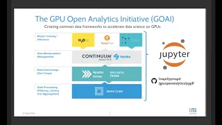
So
to
avoid
that
hue
I
initiated
was
started.
Its
GPU,
open,
analytics
initiative
and
map
t
is
a
founding
member
of
that
with
other
companies,
and
it
basically
allows
you
to
go
AI.
Actually,
the
first
project
created
a
GPU
data
frame
or
gdf.
It
basically
allows
you
to
efficiently
interchange
data
between
different
processes
running
on
the
GPU.
B
And,
as
you
can
see,
maxie
actually
system
very
well
with
the
machine
learning
pipeline,
you
know
we
accelerate
the.
You
know
the
feature
engineering
process,
basically
allowing
you
to
you
know,
identify
the
features
that
are
important.
We're
also
because
of
our
visualization
they're,
able
to
kind
of
explain
what
those
AI
models
are
doing.
C
B
Visually
showing
it
and
also
the
same
time,
you
know
when
you
have
predictions
and
you
have
the
actual
outcomes
you
are
able
to
compare
whether
your
predictions
are
in
line
with
your
actual
outcomes.
So
more
and
more
map
D
is
becoming
an
integral
part
of
any
machine
learning
pipeline
a
month
ago,
and
actually
we
launched
map
D
for
dot,
o
and
O.
B
We
actually
support
geospatial
data
types,
so
that
means
we
can
actually
support.
Any
of
these
geospatial
objects
like
a
point
line,
string,
polygon,
Multi,
polygons,
and
so
these
are
Native
now
in
the
MACD
database,
so
you
can
actually
run
the
SQL
statements
that
can
use
functions
like
ft
distance
SD
contains
which
on
this
data
set
now
this
is
this
kind
of
helps
you
in
in
displaying
this
information.
Now
where
we
were
used
to
be
able
to
do
like
just
5,000
polygons
using
the
front-end
rendering.
Now
we
can
actually
do
that.
B
So,
who
are
our
customers
map?
T
has
customers
that
includes
telcos
capital,
market
advertising,
oil
and
gas.
You
know
federal
utility,
so
it
covers
many
verticals
and
most
of
these
organizations
are
data-driven
and,
and
so
they
use
Mattie
or
operational
analytics
to
actually
drive
real-time
tactical
decisions.
When
you
know
the
data
is
coming
with
high
velocity
and
this
high
volume
data.
B
So
if
a
company
like
you
know
a
wireless
companies,
you
know
wondering
why
the
phone
updates
go
bad
or
you
know
if
they're
determining
you
know
the
patterns
in
cell
and
Wi-Fi
data,
and
all
these
have
a
geographic
component
to
it.
So
it's
very
easy
to
kind
of
find
those
patterns
and
get
really
good
insight
into
your
data
using
map
T,
and
this
can
be
done
interactively.
C
B
And
you
know
how
you
know:
businesses
are
actually
adopting
mappy
to
basically
to
exclude
around
with
you
know
the
data
that
they
have
and
it
becomes
like.
Maddie
becomes
an
integral
part
of
their.
You
know
the
data
exploration
pipeline
before
the
feed,
the
interesting
you
know,
data
point
to
their.
You
know,
AI
or
machine
learning
pipeline.
B
B
So
if
you
click
on
the
flights
demo,
for
example,
so
this
is
how
a
typical
dashboard
look
and
as
I
was
explaining,
you
have,
you
know
complex
charts
like
scatter
plot,
which
are
using
7
million
in
this
case
I'm.
This
is
much
smaller
compared
to
our
typical
customer,
which
are
in
hundreds
of
millions
or
billions
of
rows.
B
Now
you
find
a
scatter
plot,
you
know
a
choropleth
and
then
a
heat
map
again,
along
with
you,
know,
simpler
charts,
like
line
charts
and
bar
charts
and
a
table.
So
in
the
in
the
first
one,
for
example,
you
see
the
departure
delay
and
the
arrival
delay
plotted
out
and
you
see
almost
a
you
know
a
straight
line,
and
this
is
expected.
B
When
you
have
you
have
a
you
know,
delay
in
departures
that
you'll
arrive
late,
but
also
it's
color-coded
based
on
the
add
line
and
will
actually
do
this
chart
on
the
GPU
just
wanted
to
give
you
a
quick
idea,
and
then
here
in
in
the
coroplast,
you
will
notice
that
you
can
actually
zoom
in,
and
you
can
hover
over
here
and
you
notice
that
the
state
of
Illinois
is
and
state
of
New
York
actually
have
very
similar.
You
know
arrival
delays
by
destination.
B
You
can
also,
you
also
have
you
know
flights
by
month
and
day
of
the
week.
So
here
is
the
month,
and
here
is
the
day
of
the
week
and
you
notice
the
color
patterns
that
blue
means
the
fewer
flights
and
on
Saturday
is
really
as
like
as
to
be
expected.
You
know,
is
quite
low
number
of
flights
taking
off
on
Saturday.
B
Now
you
also
have
a
line
chart
which
shows
based
on
the
you
know
the
time
and
the
number
of
records.
Now
you
can
also
kind
of
drill
down
or
a
smaller.
You
know,
period
of
time
by
simply
using
dragging
you
know
on
the
lower
the
scale,
and
you
can
see
that
you
have
actually
selected
a
much
smaller
window
and
as
you,
the
most
important
thing
is,
as
you
are,
you
know,
selecting
a
certain
column
or
a
certain
timeframe.
It
gets
applied
across
all
the
charts
that
are
derived
from
the
same
table.
B
Now
you
can
actually
combine
multiple
tables
and
multiplayers
and
that's
a
different
topic,
but
that
is
a
beauty
of
you
know:
map
T,
where
I
do
a
select
on
this
on
these
fields
and
it
immediately
gets
applied
to
all
the
chart,
and
it
all
happened
so
fast
to
the
blink
of
an
eye
that
you
see
that
every
single
chart
got
updated.
So,
for
example,
if
I
click
on
United
add
lines,
you
will
notice
that
everything
got
updated
now
from
the
7
million
records
you
have
like
26,000.
B
B
B
You
know
multi
node,
you
know
with
you
know
the
gateways
and
you
know
Bastion
servers,
and
you
know
basically,
so
what
I
did
was
I
wanted
to
have
a
very
simple
deployment
with
just
three
nodes,
one
master,
and
you
know
couple
of
nodes
in
specifically
like
one
nor
the
GPU
and
one
with,
if
you
just
to
make
sure
I
conveyed.
Of
course
you
can
scale
it
out,
depending
on
your
deployment
and
I
found
sistex
tutorial
to
be
very
useful.
B
They
actually
have
a
cloud
formation
script,
which
I
borrowed
and
I
kind
of
modified
it
to
launch
this
setup,
where
I
have
a
centaur
running
on
a
t2
medium
and
that's
going
to
be
my
master
I
have
another
centaurs
running
on
a
p2
extra-large,
which
has
a
test
la
ke
GPU,
and
so
that's
going
to
be
my
GPU
worker,
node
and
I
have
a
on
at
e2
dot.
Large,
that's
going
to
be
my
CPU
worker
node.
B
Now
they're,
all
part
of
a
V,
PC
and
I
also
opened
up
the
port,
which
will
be
communicating
now
in
addition
to
that,
I
also
attached
an
EFS,
an
elastic
file
system
because
I
just
wanted
an
NFS
share.
So
I
just
mounted
I
created
an
NFS
now
make
sure
that
when
you
create
that
NFS,
that
is
part
of
the
same
V
PC
and
you
know
it
belongs
to
the
security
group.
So
that
way
you
can
communicate
now.
B
B
B
But
hopefully
these
instructions
are
still
valid
now
and
then
I
ran
to
the
Play
Books
to
prepare
the
environment,
and
you
know
one
important
thing
is
of
course
you
know,
fix
the
post
inventory
file
to
reflect
your
setup
and
again
these
instructions
that
are
you
know.
Chronicled
over
here
are
applicable
for
both
cloud,
and
this
could
be
any
cloud
or
your
on-prem
deployment.
B
And
so
once
you
run
through
the
ansible
and
everything
is
okay,
you
should
be
able
to
create
an
admin
account,
the
password
and
and
one
way
to
kind
of
smoke
that,
if
everything
is
ok
to
just
log
into
your
web,
console
opens
of
that
console.
So
most
of
my
instructions
are
using
the
command
line,
oc2
and-
and
so
that's
what
we
will
do
now
after
you
verify
whether
your
nodes
are.
Ok,
then
what
you?
What
I
did
was
I
label
the
node
so
make
sure
that
you
know
enable
it
a
CPU
and
GPU.
B
B
So
that
way,
if
I
have
to
do
some
loading
and
creating
the
tables,
I'll
use
the
CPU
version
and
keep
my
GPU
version
powered
off
and
just
to
save
some
money
and
and
then
once
I've
done
with
all
those
you
know,
tasks
then
I
I
won't
to
actually
go
and
clear
run.
The
queries
then
I
can
fire
up
the
GPUs.
In
fact,
I
can
even
use
the
CPU
version
for
creating
the
charge,
but
then-
or
actually
you
know
querying
when
then
I
could
use
the
GPU.
B
That's
when
I
really
need
the
computational
power,
and
now
one
important
note
is
the
Nvidia
driver
installation.
So
this
was
a
little
bit
involved
on
the
center
OS
and
so
I've
documented.
All
the
you
know
the
how
to
install
the
Nvidia
driver,
the
container
runtime,
how
to
set
up
the
hook
and
things
like
that.
B
B
You
know,
deploy
map,
dgq,
yamo
and,
in
this
case
I'm
just
deploying
a
pod,
maybe
in
another
blogger
sure
how
it
can
be
started
as
an
application,
service
or
deployment
where
you
have
many
copies
of
the
pod
and
you
have
an
H
a
configuration.
So
this
is
a
very
simplistic
one.
I
define
the
pod
and
I
specify
the
note
type.
There's
GPU,
and
you
know
this
is
the
the
darker
image
the
C
II
Community
Edition
CUDA
stands
for
the
GPU
elation
and
we
are
mounting
the
NFS
under
slash
map,
D
storage.
B
C
C
B
B
You
will
see
that
this
is
of
type
GPU,
so
the
dot
12
is
the
10
1000
dot.
12
is
actually
the
GPU
node.
Just
remember
that
the
dot
Phi
is
the
TP.
You
know
and
if
you
say,
OC
get
cards,
so
these
are
the
docker
containers
that
are
running
now
by
default.
These
are
the
open
shift,
management,
docker
containers,
the
registry,
the
router,
that's
all
running
and
also
the
OC
get
service.
B
B
Okay,
so
I
think
it
should
be
ready
to
go
yes,
part
if
you're
doing
it
initially,
it
might
take
some
time
because
it's
going
to
be
pulling
the
image
I
already
pulled
that
image.
So
that's
why
this
little
it's
very
snappy,
and
the
next
thing
is:
let's
make
sure
that
now
that
we
know
it's
running
on
the
12
I'm
going
to
do
an
SSH.
B
B
That
will
tell
you
whether
the
amount
of
GPU
memory
is
sufficient
or
not,
and
also
you
notice
that
in
the
process
section
you
see
that
the
map
D
server
is
running.
Now
you
can
actually
log
in
to
the
the
pod
by
simply
saying
o
CR,
SH,
mathy
and
and
boom
you're
right
there.
So
if
you
do
an
DF
edge,
you'll
notice
that
the
NFS
share
is
actually
mounted
on
slash
map
storage,
which
has
a
database,
and
if
you
look
at
the
storage.
B
B
And
it's
going
to
be
inserting
it
it's
pulling
the
CSV
file
or
the
net
and
inserting
it.
Hopefully
it
will
be
done
in
two
seconds:
okay,
it's
done,
and
next
what
we'll
do
is
I'm
going
to
fire
up
the
map,
T
command-line
utility
and
it's
called
map-
t
/
in
map
dql
and
the
default
is
database
called
map
t,
and
this
is
a
default
password
for
it,
and
you
can
see
that
it
says
user
map
be
connected
to
data
base
map
T
and
you
can
a
slash
T
to
list
the
databases.
B
Actually
I
should
have
done
this
before
we
imported.
So
when
you
initially
do
you
get
your
darker
image?
These
three
tables
are
already
there.
These
actually
have
the
polygons
for
the
different
counties,
countries
and
state.
So
that
way
you
can
do
it
join
when
you
have
you
know
your
own
data
set.
So
that
way
you
can,
you
know,
draw
the
coral
pads
and
you
know
those
kinds
of
charts
using
geographic
information.
So
we
have
the
flight
data
set
and
you
can
describe
the
data
set
by
saying
/t
flight.
B
And
it's
got
quite
a
lot
of
columns
and
actually,
in
the
blog,
what
I've
done
is
I
just
put
just
the
the
column
that
we
will
be
using
in
our
query
so
for
time.
What
I've
done
is
I'm
trying
to
do
a
cut
paste
of
this
query
that
I've
saved,
so
it's
basically
select
the
origin
city
and
the
destination
city
and
the
average
air
time
you
know
and
you're
basically
grouping
it
by
the
origin,
city
and
destination
cities
where
the
distance
is
less
than
hundred
thirty-five
miles.
And
so,
if
I.
B
It's
moving
the
data
from
the
NFS
share.
You
know
through
the
CPU
to
the
GPU.
So
that's
why
the
initial
delay
now,
if
I,
run
the
command
again,
it's
almost
instantaneous
now
now
that
it's
initially
loaded
that
column
that
you
are
operating
on
now
any
further
slicing
and
dicing
of
those
columns
are
going
to
be
in
milliseconds,
but
the
initial
load
is
going
to
come
from
your.
You
know,
persistent
storage,
and
you
will
see
you
know
much
longer
in
a
query
time.
Okay,
so
we
have
been
able
to
successfully
look
at
that
now.
B
B
B
And
as
you
can
see
in
this
case,
we
are
starting
a
service
and
we
are
exposing
the
port
9:09
to
as
3009
to
and
do
using
the
node
port
service
well
in,
in
effect,
the
port
30
90
to
30
0
92
in
that
cluster.
So,
even
though
I
can
also
use
the
public
IP
address
of
the
computer
or
the
GP,
nor,
even
though
it's
running
on
the
GPU
node,
so
let's
go
ahead
and
create
the
service.
B
B
And
voila
we
are
in
and
if
you
go
to
the
Data
Manager,
we
should
see
our
flight
2008
10k
and
you
click
on
that
and
you
notice
that
there
you
know
10,000
rows
or
56
column,
and
so
now
we
are,
we
can
go
ahead
and
you
know
do
our
puh
and
you
can
click
on
the
new
dashboard
and
you
can
click
on
add
chart
and
you
need
a
source
for
the
the
which
is
a
table.
So
we
will
select
the
flight
database
table
and
then
in
the
so
you
have
two
things.
B
One
is
that
dimension
and
another
is
a
measure.
So,
first
we
are
going
to
select
what
kind
of
chart
do
we
want.
So
we
want
to
create
a
scatter
plot,
just
right
here
and
so
I
think
that
as
I
was
mentioning
before
you
see,
a
combination
of
you
know
pretty
complex
charts
like
point
map
geo
heat
map,
choropleth,
all
of
them
using
geographic
information
and
rendered
in
the
back
in
the
back
end
by
the
GPU.
B
B
And
you
notice
that
it
immediately
renders
it.
You
can
also
choose
a
color
palette
to
decide
what
else
you
want.
Basically,
the
difference
between
the
measure
and
the
dimension
is
the
dimension
is
the
categories.
So
this
is
typically
your
roll
label
in
a
table
and
the
measures
are
actually
the
aggregated
values,
like
you
know
the
sum
average
and
all
that-
and
this
is
basically
a
column
in
a
table.
So
now,
once
you
create
the
chart,
you
can
say
apply
and
that
creates
it
and
then
you
can,
you
know,
give.
B
B
Of
course,
the
termination
takes
a
few
seconds,
so,
let's
pause,
while
it's
terminating.
What
we're
going
to
do
is
we
are
going
I'm
going
to
do
a
cat
of
deploy
map
DCP,
you
not
llamo,
so
this
is
a
mo
file
that
we'll
use
for
deploying
the
CPU.
What's
the
main
difference
here,
the
main
difference
here
is
the
node
type
is
CPU
and
the
image
that
I'm
going
to
use
is
map
the
community
edition
you
we
are
going
to
use
the
same
amount
point
coming
from
our
NFS
server.
B
C
B
The
way
have
you
update
or
geospatial
that
was
launched
yesterday
so
looks
like
we
have
a
newer.
You
know.
Docker
images
took
a
while
to
pull
okay,
so
that
should
be
in
a
ready
state
now
and
it's
a
is
running
so
now.
I
can
say:
OC
create
minus
F
map,
D
service,
dot,
yeah
mo
and
so
services
created.
So
in
fact,
I
should
be
able
to
go
to
the
same.
B
B
B
A
A
C
A
Put
the
query
in
that
Miss:
that's
good,
but
definitely
cross
link
to
the
blog
post
when
I
post
this
up
on
YouTube
and
on
online
OpenShift,
well,
I'm
looking
to
see
if
there's
any
questions,
I'm
curious
to
see,
if
there's
other
people
who
are
already
using
the
map
D
who
are
on
the
call
or
who
watch
this
video
and
if
now
they're
thinking
of
deploy
on
open
ship
if
they
could
reach
it,
I'd
love
to
see
and
hear
you
know,
get
feedback
on
it.
Both.
B
A
B
C
B
A
Also
give
a
shout
out
to
the
machine
learning
on
openshift
special
interest
group,
which
means
the
first
Friday
of
every
month
and
tomorrow
there
will
be
one
if
you
go
to
Commons,
OpenShift
org
and
look
at
the
events
calendar.
All
the
details
are
there
and
we
have.
You
know
lots
of
lots
of
each
each
week.
We
have
a
couple
of
folks
give
very
short
presentations
and
there's
a
lot
discussion
about
different
use
cases
and
best
practices
for
running
these
ml
and
other
workloads
on
on
openshift
and
kubernetes.