►
From YouTube: IETF102-ANRW-20180716-1330
Description
ANRW meeting session at IETF102
2018/07/16 1330
https://datatracker.ietf.org/meeting/102/proceedings/
A
A
D
Well,
so
we
were
very
hopeful
that
would
happen,
and
we
very
much
want
to
have
you
participate
in
both
the
IRT
F
and
the
IETF.
So
if
you
have
any
questions
about
processes
feels
please
feel
free
to
talk
to
me,
I'm
also
a
long
time,
ITF
er.
Let
me
turn
it
over
to
our
session
chair
now
and
enjoy
the
afternoon.
C
B
Thank
You
Philippa
hi
everyone.
This
talk
is
about
thinking
beyond
binary
failures
in
network,
so
when
we
think
about
network
equipment
like
links
and
routers,
we
normally
think
of
them
as
having
a
binary
state
like
on
or
off
or
up
and
up
or
down,
and
what
I
want
to
tell
you
today
is
that
there's
actually
a
ritual
that
exists
in
between
and
if
you
embrace
that
world
and
there's
a
lot
of
benefits
in
terms
of
efficiency
that
we
can
have.
But,
first
of
all,
why
do
we
care
about
having
efficient
networks
in
the
cloud?
B
The
idea
is
that
computing
is
in
fact
shifting
to
the
cloud
with
the
existence
of
Internet,
of
Things
and
machine
learning,
algorithms
like
autonomous
driving,
there's
a
flood
of
data,
intensive
workload
that
is
headed
to
the
world's
data
centers
and
in
fact
it's
predicted
that
the
cloud
datacenter
traffic
is
going
to
grow,
to
20
1
to
up
to
15
that
the
bytes
appear
in
just
the
three
years
from
now.
So
as
part
of
this
significant
change,
we're
building
the
cloud
infrastructure.
B
So,
like
a
new
exercise,
we
are
building
data
centers
across
the
world
with
massive
compute
power
and
we're
using
fiber
optics
cables
to
interconnect
these
data
centers
to
each
other
under
the
sea
and
across
the
mountains
right.
But
connectivity
is
extremely
important
in
the
cloud
infrastructure
and
so
there's
a
lot
of
redundancy
to
make
sure
that
the
network
is
always
connected
and
whatever
I
tell
you.
B
So
one
of
the
key
factors
that
impact
the
efficiencies
of
networks
or
link
failures
right
link
failures
are
important
in
terms
of
capacity
provisioning,
which
means
that
how
much
capacity
are
we
going
to
put
in
our
network
when
something's
false,
so
that
we
can
serve
the
rest
of
the
traffic?
Another
factor
that
affecting
link
failures
effects
is
traffic
engineering
traffic
engineering
means
once
you
built
a
network.
How
are
you
going
to
route
traffic
during
failures
these
to
feed
each
other
and
they
form
inform
each
other
as
well?
B
So
they
talk
is
about
analytics
and
optimizations
to
improve
the
efficiency
of
the
cloud
by
meant
by
making
link
failures,
not
be
binary
events.
What
do
I
mean
by
that?
Let
me
just
give
you
a
high-level
idea
of
the
talk.
What
I'm
showing
here
is
that
the
quality
of
a
typical
optical
signal
in
in
the
network,
the
Korea
region,
is
where
the
link
is
open
and
the
road
region
is
where
the
link
is
down.
B
Okay,
so
the
state
of
the
link
is
binary,
but
when
you
look
at
the
quality
of
the
signal,
it
actually
has
a
rich
behavior,
it's
not
a
binary
variable,
and
so,
when
I'm
sure
that
this
impacts
capacity
provisioning,
it
impacts
availability
of
the
links
it
also
matched
traffic
engineering,
and
so
the
high-level
idea
of
the
talk
is
that
we
advocate
for
links
that
have
adaptive
capacity
and
adaptive
reliability,
levels
but
okay.
Why
hasn't
anybody
done
this
before,
because
it's
kind
of
challenging
to
do
this?
B
First
of
all,
we
have
to
understand
the
optical
layer
characteristics
a
lot
of
the
design
that
has
been
done
for
our
based
on
worst-case
assumptions
with
lab
experiments,
and
this
is
the
first
time
that
we're
looking
at
the
quality
of
optical
signals
in
the
world
for
a
long-term
study.
Secondly,
we
need
some
sort
of
a
reconfigurable
Hardware
that
is
capable
of
switching
between,
but
when
you
do
different,
very
different
variables
and
we
need
an
infrastructure
that
does
all
of
these
measurements
right.
Third,
this
is
a
significant
change.
B
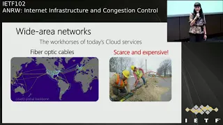
What's
the
right
area
network,
it's
a
network,
a
interconnects
major
cities
together,
it's
basically
the
workhorse
of
today's
cloud
services
and
most
of
the
major
cloud
service
providers
like
Google
Microsoft,
Amazon
Facebook.
They
are
using
fiber-optic
cables
to
interconnect
these
major
cities
together,
but
it
turns
out
that
putting
fiber
under
the
ground
and
over
the
mountains
and
whatnot
it's
kind
of
a
laborious
task,
so
fiber
is
expensive
and
a
scarce
resource
right.
B
B
These
are
the
devices
that
sit
in
major
cities
and
they
can
read
the
optical
and
electrical
signal
to
each
other,
and
then
the
red
lines
are
the
fiber-optic
things
it
feed
them
to
enable
long
reach
every
50
miles
or
so
there's
an
amplifier
device
that
sits
in
between,
and
so
this
study
contains,
50
of
these
optical
cross
connect
devices
say
in
50
major
cities
about
a
hundred
of
these
fiber
segments
and
about
a
thousands
of
these
amplifier
devices.
Okay,
I
wanna
zoom
into
one
of
these
fiber
links
to
get
a
better
idea
of.
B
What's
going
on
so
on.
One
side
on
the
red
line
is
a
fiber
link
and
on
the
two
sides
I
have
these
devices
optical
cross
connects
it's
actually
two
different
fibers
for
a
different
path
and
there's
these
optical
channels
or
wavelengths
that
are
traveling.
A
signal.
Okay
and,
like
I,
said:
there's
this
amplifier
notes.
These
amplifiers
notes
add
noise
to
the
signal
and
they
can
fail
independent
of
each
other.
B
So,
from
a
router
with
respect,
if
I'm
an
IP
layer
perspective,
think
of
the
routers
are
connected
to
the
optical
cross
connects
and
then
there's
a
device
called
the
transponder.
This
transponder
translate
the
signal
between
the
electrical
and
optical
domains
and
depending
the
bitrate
of
the
transponder,
the
bit.
The
capacity
of
the
link
basically
depend
on
the
modulation
of
this
transponder.
So,
for
example,
we
were
studying
hundred
gigabits
per
second
wavelengths
or
because
it's
per
second
channels
that
use
qpm
QPSK
modulation.
B
This
means
that
the
signal
is
programmed
to
carry
100
gigabits
per
second
of
traffic.
Okay,
in
totality
picture
that
a
map
of
the
north
america,
I
will
show
you
we
are
studying
2000
channels.
That
means
about
200
therapies
per
second
of
capacity,
so
typically
there's
a
one-to-one
mapping
between
one
of
these
wavelengths
and
one
IP
layer
links.
So
every
time
that
I'm
saying
in
the
wavelength
or
a
channel,
I'm
gonna.
Think
of
a
one
port
of
these
routers
on
one
IP
layer
link.
B
Okay,
let
me
show
you
how
it
looks
like
so
on
the
x-axis
I
have
time,
I,
don't
know
why
axis
I'm,
showing
you
signal-to-noise
ratio,
signal-to-noise
ratio
is
a
standard
metric
to
measure
the
quality
of
an
other
signal,
the
higher
the
signal-to-noise
ratio,
the
better
the
quality
of
the
signal,
there's
also
a
threshold
on
the
signal-to-noise
ratio
has
to
be
above
that
threshold
for
the
link
to
be
up
to
be
considered
up.
So
above
the
threshold,
the
link
is
out
by
IP
layer
link
is
up
and
below
the
threshold.
The
link
is
down.
B
The
optical
link
is
that
IP
IP
layer
link
is
also
down.
Okay,
so
signal
is
kind
of
stable,
but
it
also
has
these
little
tips
there
too
right.
So,
what's
going
on
in
these
tips,
I'm
just
zooming
into
one
of
them.
You
see
the
link
is
still
up
it's
in
the
green
area.
It's
about
two
and
a
half
hours
on
average.
B
These
dips
that
lasts
about
four
hours
and
the
quality
has
degraded
a
little
bit,
but
the
link
is
still
up
okay,
so
it
turns
out
that
some
of
this
is
just
collateral
damage
caused
by
humans.
So
this
is
one
of
those
amplifier
huts
in
a
Seattle
area
where
fiber
is
coming
up
from
the
ground
and
it's
being
amplified
or
new
babies
are
being
added
or
deleted.
B
What
seems
to
be
happening
is
that
humans
going
to
working
on
one
of
these
fiber
tips,
but
then
the
fiber
is
super
sensitive
to
head-to-head
connectivity
and
if
somebody's
opening
up
the
cabinet's
door
or
they
like
working
on
something
underneath
and
then
something
somebody
hits
another
fiber,
then
they
disrupt
the
connectivity,
not
so
much
so
that
their
link
is
disconnected,
but
sometimes
they
disrupt
their
connectivity
in
such
that
SNR
drops
and
then,
after
a
couple
of
hours,
now
they're
done
with
their
work,
they
come
backs
or
somebody
fixes
it.
And
then
it
comes
back.
B
Ip
layer
doesn't
see
this,
but
are
the
optical
layer
can
see
it.
So
this
is
the
threshold
for
for
caring
hundred
gigabits
per
second
of
data.
Okay
is
that
I'm
gonna
show
you
the
threshold
of
caring,
different
amount
of
capacity
having
different
amount
of
capacity
on
this
link
so
see
because
we
wanted
to
avoid
these
dips.
B
In
the
signal
we
chose
a
hundred
gigabits
per
second
modulation
as
a
fixed
modulation,
so
that
we
sort
of
not
hate
too
many
of
these
little
dips
in
the
link,
and
what
I'm
gonna
argue
is
that
well
what
if
we
were?
We
were
carrying
150
units
per
second
of
data,
whatever
using
a
higher-order
modulation
for
this,
it
would
have
been
hitting
a
few
more
of
these
dips
in
a
signal-to-noise
ratio,
but
you
know
we
would
have
been
carrying
also
50
kilo
bits
per
second
more
data.
B
Another
point
I
want
to
make
is
look
at
this
point
right
here
with
the
circle
normally
right
now.
This
is
a
failure,
because
the
signal
to
noise
ratio
is
under
200
gigabits
per
second
capacity.
However,
it's
above
50
gigabytes
per
second
capacitance.
So
it's
not
a
total
failure.
I
could
have
been
carrying
50
gigabits
per
second
of
data,
had
I
had
the
capability
of
switching
between
these
different
speeds.
B
So
basically
the
takeaway
is
that,
because
we're
thinking
of
failures
as
pioneering
events,
there
is
wasted
capacity
in
the
way
that
we
are
carrying
data.
There's
also
missed
opportunities
to
keep
the
link
up.
While
we
could
have
been
care
keeping
it
up,
and
when
we
look
at
the
fillings,
all
of
those
2000
different
channels
and
whatnot,
we
notice
that
there's
actually
a
wide
difference
across
channels.
Not
all
of
the
channels
are
going
to
look
like
this,
not
for
not
all
of
them.
B
150
user
bits
per
second
is
the
best
choice,
and
so
there's
the
main
idea
that
we
want
to
advocate
is
to
enable
adaptive
links.
So
the
challenges
are
well.
Of
course
we
have
to
quantify
impact.
Secondly,
we
have
to
sort
of
change.
The
traffic
engineer,
optimization
algorithms,
that
we
and
we
have
to
have
reconfigurable
Hardware
remember-
is
that
I'm
just
going
to
cover
the
first
one,
the
quantifying
impact
and
I
refer
you
to
our
upcoming
second
paper,
this
August
on
the
rest
of
the
details.
B
Okay,
the
median
is
actually
predict,
so
SNR
is
higher
than
the
threshold,
which
is
good,
but
it's
way
too
good.
The
median
is
7
DB
higher
than
what
is
supposed
to
be,
and
not
only
that
but
99%
over
the
time.
The
channel
quality
is
higher
than
the
threshold
450
years
per
second,
so
kind
of
99%
of
the
time
I
could
have
been
carrying
150
years
per
second
of
traffic
and
43%
of
the
time
I
could
have
been
carrying
200
kilobits
per
second
of
traffic.
So
this
means
that
there
is
this.
B
B
Had
I
had
a
way
of
switching
to
fifty
yards
per
second
okay,
when
we
looked
at
all
of
these
links
together,
what
we
saw
was
that
availability,
which
is
the
amount
of
time
that
each
of
these
links
are
spending
in
the
green
region,
is
also
totally
different,
so
here
I'm
showing
the
availability
percentage
of
all
of
these
links
as
a
as
a
CDF.
That's
a
cumulative
distribution
function
and
the
actual
number
really
doesn't
matter.
B
What
matters
is
that
there's
a
wide
difference
between
these
channels,
but
there's
four
different
phone
nights
from
five,
not
from
99.999
to
ninety
percent,
and
we
we
made
a
similar
observation
in
terms
of
time
to
repair
and
failure.
Probability
for
these
different
things.
What
I'm,
showing
here
is
somewhat
of
a
similar
graph
but
I'm
calling
the
failure
probability
of
different
links.
So
what
does
this
mean?
This
means
that
this
would
impact
traffic
engineering.
Okay.
Why?
B
Because
traffic
engineering
is
the
function,
is
the
algorithm
that
is
configuring,
the
allocation
of
traffic
on
different
paths
right,
and,
if
you
don't
understand,
if
you
don't
think
about
the
different
probabilities
of
different
links
failing
then
we
are
making
its
uniform
an
assumption.
So
the
goal
of
traffic
traffic
engineering
is
to
maximize
the
performance
while
utilizing
the
resources
of
the
network
that
matching
that
are
matching
the
current
demand
right.
So
it's
a
periodic
effort.
B
It's
been
a
subject
of
extensive
research
in
in
Prior
work,
but
the
most
important
thing
about
traffic
engineering
is
that
we
have
to
do
traffic
engineering
on
your
failures
right.
What
I
want
to
make
it
make
a
case
for
is
that
prior
work
optimizes
for
the
worst
case,
but
the
problem
is
that
we
end
up
excessively
over-provisioning
the
network,
because
we
want
you
to
if
you
wanna,
we've
sort
of
one
of
withstand
shifts
in
traffic
during
failures,
but
there
may
be
improbable
failures.
B
B
So
if
the
toppling
fails
and
the
bottom
link
fails,
I
would
like
to
my
network
to
be
able
to
carry
the
entire
traffic,
hence
I'm
going
to
carry
10
gigabits
per
second
all
the
time,
because
even
when
the
links
haven't
failed,
I
would
like
these
two
links
to
be
by
standing
as
as
backups,
and
so
this
is
what
happens
really
in
practice.
I'm
showing
the
traffic
on
two
links
and
on
August
4th
one
of
the
links
has
failed.
The
blue
link
has
failed
and
the
entire
traffic
has
shipped
with
your
orange
link.
B
Ok,
and
so
what
is
happening
is
that
if
I
extend
this
graph
to
the
left
and
to
the
right,
the
orange
link
has
the
capacity
of
carrying
that
much
traffic,
but
it's
not
because
it's
just
as
a
standby
of
the
a
of
the
blue
link.
So
what
we
advocate
for
is
that
we
advocate
to
use
failure,
probabilities
of
each
link
to
reason
about
the
likelihood
of
different
failure.
Events,
and
so
in
this
case,
how
do
I
have
these
failure?
Probabilities
from
the
optical
domain,
I
would
have
said.
B
Ok,
I
can
just
use
a
probabilistic
guarantee
about
this
network.
I
can
just
carry
10
zero
on
the
most
probable
link
to
fail,
and
then
we
I
can
carry
20
gigabits
per
second
99.99%
of
the
time.
So,
given
basically
an
uncertainty
vector
I'd
like
to
come
up
with
an
allocation
vector
keeping
a
floor
demand
between
these
these
sources
and
estimations
such
that
I
can
say
well
fall
of
the
flow
is
95%
of
the
time.
The
demand
is
satisfied,
99.99%
of
the
time
and
I
can
make
it
statements.
B
Like
loss
would
be
less
than
5%
of
the
of
the
demand
99.9
percent
of
the
time,
I'm
gonna
skip
the
details
of
the
traffic
engineer
algorithm
and
put
everything
together
for
you.
Okay,
what
I'm
advocating
for
is
using
per
channel
signal-to-noise
ratio
and
failure.
Probabilities
alongside
flow
demands
on
floor
routes
for
traffic
engineering
flow
demands
on
floor
rats
are
coming
from
the
IP
layer.
This
is
how
we
do
traffic
engineering
today.
The
pressure
on
all
signal-to-noise
ratio
and
failure.
E
Robert
Robert
Cisco
Systems,
a
very
nice
thought.
Thank
you.
The
per
channel
SNR
I'm
wondering
if
there
might
be
analogs
in
the
RF
space
right,
because
it's
if
you're,
basically
presenting
effectively
an
RF
space
where
you're
getting
some
effective
bit
throughput
and
one
could
imagine
the
per
channel
failure
probability.
Something
like
that
separate
from
changing
modulation
schemes.
Doing
an
error
correcting
that's.
B
A
very
great
observation:
yes,
yes,
the
answer
is
yes
and
there's:
there's
working
your
wireless
wireless
domain
and
RF
the
way
one
of
the
differences
between
the
optical
domain
and
RF
domain
is
that
actually
we
can
read
as
an
RPD
accurately
and
as
an
R
does
not
change
as
quickly
as
snr
changes
in
wireless
signal,
the
the
measurements
that
we're
restoring
yours
every
15
minutes,
and
when
we
looked
at
this
in
it
15
minutes.
Yes,
not
actually
doesn't
change
that
much
time
scale
it
on
presenting
it's
longer,
so
it's
kind
of
better
actually,
for
this.
B
B
Question
yeah
yeah,
so
I'm
still
analyzing
the
data.
My
hunch
is
that
most
of
the
failures
are
because
of
the
failures
on
the
transformer
size
which
means
per
channel,
but
there's
definitely
something
as
when
the
amplifier
fails
most
likely
most
of
the
channels
together
fail
or
when
there's
a
fiber
cut
all
of
the
channels
together
fail.
So
I
don't
have
a
concrete
answer
for
that
yet.
But
my
hunch
says
there
there's
significant
number
of
failures
that
are
happening
on
the
transporter
site,
which
is
a
channel
failure.
So.
F
B
G
B
That
question,
so,
if
it's
on
the
fiber
side,
it
means
that
the
probability
of
failures
would
be
a
different
number.
We
may
not
be
able
to
change
the
capacity
because
things
have
failed
if
there's
no
fiber,
if
there's
no
fiber,
but
we
can
allocate
the
failure
probability
correctly
when
we
are
designing
the
network.
So
you
know
a
fiber
in
Brazil
may
have
a
higher
probability
of
failure
than
than
a
fiber
somewhere
in
the
middle
of
the
US,
and
so
with
that
we
can
inform
traffic
engineering
and
capacity
provisioning
by
just
measuring
these
probabilities.
H
B
I,
don't
think
much
would
change
what
I
was
telling.
You
was
to
sort
of
make
a
mental
model
that
when
I'm
showing
you
one
of
these
graphs,
it
could
be
one
I
peeling,
but
let's
assume
that
it's
two
I
peeling.
So
what
it
means
is
that
that
capacity
of
these
two
IP
links
can
be
increased
so
in
the
traffic
engineering
optimization.
If
you
have
a
in
between
them,
then
the
the
sort
of
the
engine
should
take
care
of
it
sure.
G
Rami
from
Case
Western,
Reserve,
University,
so
I
have
a
question.
When
you
looked
at
their
channel
as
a
nod,
did
you
consider
the
distortion
introduced
by
the
amplifiers,
because
the
more
amplifiers
that
the
signal
or
the
chair
or
the
signal
is
going
is
through
the
more
distortion
that
will
be
introduced
by
those
you.
B
I
I
All
right,
so
climate
change
is
perhaps
the
most
significant
problem
facing
humanity
today,
and
you
know
when
we
talk
to
different
people,
they
come
up
with
different
definitions
right
all
of
them.
They
refer
to
global
warming
as
simply
climate
change.
But
then,
when
you
talk
to
the
real
climate
scientists,
they
say
that
it
is
not
just
a
global
warming,
but
it
actually
encompasses
a
number
of
things
that
could
have
significant
effects
on
the
parrot
and
these
effects
could
range
from
or
drastic
increase
in.
I
Temperatures
to
you
know
having
a
lot
of
droughts
and
heat
waves,
and
you
know
all
the
Hurricanes
that
we
might
see
in
the
future
will
be
more
and
more
intense
as
well.
As
you
know,
a
combination
of
heat
waves
and
extreme
temperatures
will
lead
to
you
know,
effects
like
false
fives,
but
one
of
the
significant
problems
that
we
will
face
in
the
future
is
the
increase
in
sea
level
rise.
I
As
you
know,
things
warm
in
the
planet
because
of
global
warming
and
other
drastic
effects,
Arctic
ice
caps
and
polar
ice
caps,
their
melt
and
they're
going
to
lead
to
increase
in
sea
level
rise,
and
this
is
a
slide
taken
from
NASA.
This
was
published
in
2014
I
want
to
like
point
to
one
key
point
shown
in
the
slide,
which
is
you
know.
We
know
seas
are
racing
and
we
know
why,
but
the
urgent
questions
are
by
how
much
and
how
quickly
alright.
I
Since
then,
people
have
been
working
on
a
number
of
models
in
terms
of
understanding
the
impact
of
sea
level
rise
on
different
things
and
and
based
on
the
model
that
has
been
developed
by
NASA
and
some
of
the
researchers
in
the
space.
You
know.
The
main
question
we
want
to
ask
in
this
talk
is:
what
is
the
impact
of
climate
change,
induced
sea
level
rise
on
the
Internet
infrastructure?
Ok,
before
you
know
answering
this
question,
we
want
to
first
look
at
weather,
see
what
are
actually
a
problem
to
the
Internet
infrastructure.
I
So
what
we
found
from
some
of
the
studies
that
have
you
know
proceeded
in
this
place
is
that
entities
like
water,
ice
and
humidity.
They
are
actually
indeed
threats
to
the
fiberoptic
stance
and
that
could
lead
to
a
host
of
problems
like
signal
loss,
attenuation,
physical
damage
like
corrosion,
fiber,
breakage,
etcetera
and
based
on
our
experiences
in
terms
of
physical
topology
mapping.
Over
the
years,
we
actually
make
two
key
observations.
I
You
know,
do
a
fix
like
inundation
and
corrosion,
and
this
aging
will
only
magnify
and
aggravate
the
effect
of
climate
change
and
the
sea
water
on
the
Internet
infrastructure.
Okay.
So
how
do
we
analyze
the
problem?
So
we
take
two
different
data
sets
to
analyze
this
problem
or
the
impact
of
sea
water
on
the
Internet
infrastructure.
The
first
one
is
the
infrastructure
data
from
the
internet
Atlas
project,
which
is
by
far
the
largest
repository
of
the
physical
Internet
data
out.
I
There
say
we
have
maps
of
over
a
thousand
four
hundred
service
providers,
from
which
you
know
we
collect
the
node
and
link
information.
So
the
node
information
include
things
like
point
of
presences,
internet
exchange
points,
colocation
facilities,
submarine,
cable
learning
stations,
etcetera
and
the
link
details
include
things
like
the
long
haul
Metro,
as
well
as
submarine
cable.
That
connect.
You
know
all
these
submarine
cable
learning
stations,
so
this
is
the
first
data
set
and
then
to
get
the
impact
of
the
seawater
and
analyze
the
impact
of
sea
water.
I
I
Coastal
geography
areas
in
all
these
course
because
of
sea
level
rise
and
they
actually
categorize
the
data
into
three
different
types,
meaning
high
low
and
medium
risk,
and
what
we
see
in
this
table
below
is
simply
the
model
of
worst-case
risk
that
could
happen
over
the
span
of
the
century.
Okay,
so
in
2030
we
would
see
about
1
feet
of
sea-level
rise
according
to
the
worst
case
model,
whereas
by
then
that's
essentially,
it
will
see
6
feet
of
sea-level
rise
in
many
of
the
coastal
areas.
I
All
right
using
these
two
data
sets,
we
analyzed
the
impact
force.
So
we
start
with
the
infrastructure
inundation
analysis
where
we
fuse
that
the
assets
using
the
projection
and
transformation
tool
using
the
ArcGIS
software,
which
is
a
geographic
information
system
that
you
know
all
the
cartographer
and
geographers
routinely
used
to
do
mapping.
I
So
the
question
you
wanna
pose
is
okay:
what
is
the
impact
of
sea
water
and
race
and
inundation
because
of
sea
water
on
the
assets
deployed
in
many
of
the
coastal
areas?
All
right?
So
the
slide
here,
which
is
gonna
pop
up
in
a
second,
actually
shows
the
whistle
overlap
between
sea
water
in
many
of
the
zoomed
in
parts
of
the
United
States
and
the
Internet
infrastructure
in
those
areas
where
the
blue
shades.
Here
they
are
actually
the
incursions.
That's
going
to
happen.
The
worst
worst
case
in
question.
I
That's
going
to
happen
because
of
the
model
predicted
and
the
assets
have
shown
in
different
colors.
So
red
actually
shows
the
submarine
cable
stations
along
with
cables
and
the
green
dots.
They
denote
point
of
presences
ix
piece
and
the
black
lines.
They
denote
long-haul
cables
and
the
green
lines
again
denote
the
Metro
fiber
deployments
in
many
of
these
areas.
Okay
visually.
We
can
actually
observe
that
this
is
a
possible
scenario
in
many
of
the
coastal
areas
in
the
US.
I
So
let
us
perhaps
you
know,
quantify
the
effect
in
many
of
these
areas.
So
what
we
do
is
we
develop
a
overlap
model
using
the
two
different
data
sets,
and
then
we
develop
a
metric
called
coaster.
Coastal
infrastructure
risk
metric,
which
is
used
to
highlight
the
amount
of
geographical
overlap
between
these
two
datasets.
I
In
many
of
the
coastal
areas,
okay-
and
we
temporarily
assess
based
on
the
temporal
patterns
given
in
the
SLR
radio
set
using
the
OLAP
tool
where
we
calculate
the
number
of
nodes
and
the
fibre
miles
that
overlap
with
the
sea
water
incursion
given
by
the
data
set.
Okay
and
basically
that's
going
to
give
it
a
bunch
of
patches
in
many
of
the
coastal
areas
where
we
simply
apply
a
kernel
density
estimate
and
then
that's
going
to
emit
a
floating-point
number
which
we,
you
know,
reverse
thought
and
then
rank
all
the
different
places,
the
risks.
I
So
the
law
here
shows
the
similar
result,
but
for
the
fiber,
conduit,
part
and
x-axis
again
shows
the
span
of
years
and
the
y-axis.
They
show
the
raw
fiber
miles
that
will
be
affected
for
long-haul
Metro
and
somewhere
in
cable,
and
what
we
see
here
is
as
high
as
2
point
6
km
miles
of
Metro
fiber
in
many
of
the
coastal
areas
will
be
affected
by
the
worst-case
syllable
rise
by
the
end
of
the
century.
I
So
the
the
next
slide
here
shows
the
same
result
for
the
link
dataset,
where
the
the
overlap
of
link
assets
in
many
of
the
geography
areas.
That
is
again
rank
is
presented
here
and,
as
you
can
see,
New
York,
Miami
and
Los
Angeles
are
like
present
across
both
those
columns
and
here's,
a
pictorial
representation
of
both
New
York
and
Miami.
Where
again,
the
blue
shades.
They
represent
the
sea
water
inundation
in
many
of
these
areas,
and
the
assets
are
shown
in
green
and
black.
I
So
as
I
can
visually
see
that
you
know
a
lot
of
Metro,
fiber
and
infrastructure
in
these
areas
will
indeed
be
under
water
over
the
coming
years.
And,
finally,
here
the
top
10
providers
I,
would
like
to
talk
to.
You
know
people
from
from
the
zoom.
You
know
if
one
of
these
powerless
and
the
room
so
so
these
are
the
top
10
providers
who
will
be
like
affected
because
of
the
deployments
in
many
of
these
areas.
I
Based
on
our
analysis,
so
our
analysis
is
actually
like,
very
very
preliminary
and
in
conservative,
in
the
sense
that
we
just
take
two
different
data
sets,
and
then
we
assess
the
overlap
between
these
two
data
sets.
But
you
know
for
those
of
us
who
believe
in
climate
change
and
how
do
we
mitigate
them?
There
are
a
number
of
steps
that
we
should.
You
know,
work
on
and
I
want
to
talk
about,
some
of
them
in
the
upcoming
slides.
The
first
thing
you
wanna
do
is
expand
the
vulnerability
assessment
that
we
have
in
this
study.
I
For
instance,
we
just
you
know,
like
I
said
we
take
two
data
sets
and
then
we
apply
overlap
and
then
you
know
come
up
with
a
set
of
risk
metrics.
So
how
do
we
incorporate
all
the
dynamic
aspects
like,
for
instance,
climate
changes
accompanied
accompanied
by
thunder
storms
and
hurricanes
and
earthquakes?
So
what
is
the
combined
effect
of
all
these
natural
disasters
on
the
Internet
infrastructure
in
many
of
the
coastal
areas?
I
I
Another
aspect
of
our
mitigation
is
to
look
at
ways
in
which
you
know:
how
do
we
integrate
the
traffic
engineering
with
risk
aware
mechanisms
from
the
ciear
metric
that
we
have?
For
instance,
you
know:
can
we
feed
the
sea
air
metric
directly
into
the
routing
substrate
so
that
we
can
redirect
traffic
in
the
face
of
such
an
outage
or
in
the
face
of
a
combined
outage,
like
thunderstorm
plus
sea
level
rise,
and
we
also
want
to
assess
the
impact
of
hardening
infrastructure
in
many
of
the
coastal
areas?
I
For
instance,
if
we
have
sea
walls
near
all
those
colocation
facilities
that
terminate
near
a
landing
station,
would
you
know
this
help
in
mitigating
the
problem
of
it?
So
we
want
to
work
on
that
aspect
as
well
and,
finally,
in
terms
of
ISP
deployments.
You
know,
apart
from
considering
metrics
like
cost
and
revenue,
and
you
know
maximizing
the
users.
J
A
J
E
K
E
L
N
C
K
K
Dines
customers
sort
of
couldn't
be
reached
because
users
were
not
able
to
get
a
mapping
between
the
name
and
the
IP
address.
So
there's
the
first
thing
that
sort
of
started
me
thinking,
oh
well,
maybe
the
DNS
isn't
as
robust
is
as
I
thought
and
then
I
strew
this
plot
as
part
of
another
bit
of
our
work,
and
this
is
a
completely
boring
line.
K
The
second
line
that
I'm
gonna
draw
is
the
one
that
sort
of
caught
my
attention,
and
this
is
the
number
of
a
wreck
that
I
found
in
the
zone
files
and
that
has
a
little
bit
of
a
different
shape
to
it
right,
because
that
comes
down
and
so
I
started
thinking,
wow,
we're
sort
of
serving
more
stuff
with
less
name
servers
right
and
there's.
Lots
of
you
can't
really
draw
that
conclusion
from
this
plot.
K
Necessarily
there's
lots
of
more
analysis
that
you
would
have
to
do,
but
a
sort
of
I
like
to
think
of
this
is
an
objective
inkling
right.
This
gives
me
some
notion
that
there's
something
to
look
at
here
and
so
I
thinking
about
sort
of
how
robust
is
the
DNS
and
I
keep
coming
up
with
sort
of
two
answers
to
this
question,
and
the
first
one
is
I
keep
coming
back
to
well,
it
must
be
good
enough
cuz.
They
never
have
any
problem
with
it.
I
use
it
every
day.
You
use
it
every
day.
K
D
K
As
I
was
thinking
about
this
more
its
thought,
well,
how
do
I
define
robustness
right?
What
does
it
mean
to
be
robust
and
that'll
make
your
head
swim
right,
because
there's
a
zillion
different
aspects
to
DNS
robustness
right,
but
the
room
that
I've
been
thinking
about
the
most
is
sort
of
can
I
sort
of
always
get
to
an
authoritative
server
for
the
record
that
I
want?
Okay.
So
that's
that's
what
T?
What
I
want
you
to
keep
in
mind
here
for
a
minute
and
I
want
to
start
here?
K
Thinking
about
that
that
notion
with
the
DNS
hierarchy
that
we
all
know
this
is
this
is
the
one
that
I
show
in
networking
class
when
I
teach
networking
right.
So
this
is
basic
stuff,
but
I
want
to
think
about
these
top
two
levels
here.
First,
the
root
and
the
top
levels
domains
right,
I
want
to
think
about
robustness
there.
K
So
this
is
community
infrastructure
up
here
we
have
things
like
lots
of
named
replicas
right,
13
named
root
servers,
so
if
I
can't
get
to
be
root,
I'll
try
J
root
or
something
okay,
I
have
lots
of
different
things
to
choose
from,
and
not
only
do
I
have
a
bunch
of
named
replicas
here,
but
I
have
lots
of
unnamed
replicas
right.
We
use
any
cast
up
here.
Most
of
the
roots
are
any
guest,
so
there's
lots
of
instances
of
J
root
or
whatever
right.
K
So
we
get
a
lot
of
robustness
up
here
at
the
very
top
of
the
hierarchy,
just
from
replicating
things
like
a
lot
okay,
so
we
can
sort
of
always
get
what
we
want,
because
there's
always
another
on
replica
there.
They
started
reasoning
about
the
next
level
here,
the
second
level
domains-
and
here
this
is
different.
It
went
often
looked
in
the
again.
The
ComNet
and
org
zone
files
and
80%
of
the
SLDS
have
two
or
fewer
authoritative
servers
named
in
the
zone
files.
Okay,
so
that's
a
lot
different
than
13
root
servers.
K
Okay,
we
know
there's
any
caste
Q's
down
in
this
level.
I,
don't
know
that
we
know
how
much,
but
we
know
that
some
of
these
domains
are
run
by
the
cloud
flares
into
their
signs
and
Bay's
anycast
and
that's
great.
We
also
know
that
there's
some
things
like
berkeley.edu
that
don't
use
any
castrate,
so
there's
some
unevenness
to
that.
K
See
how
it
looks
so
to
do
this.
These
two
basic
data
sets
I
used
the
comm
net
and
orgs
own
files
and
I
intersected
those
with
the
Alexa
list
of
popular
websites.
So
I
just
took
out
everything
from
the
zone
files
that
pertain
to
one
of
the
top
million
sites
and
put
that
in
what
we
call
a
winner
zone
file
I
did
that
once
a
month
for
the
last
nine
years.
Okay,
so
we
have
Alexa
data
going
back
nine
years
we
have
zone
file
data
going
back
nine
years.
Just
did
one
snapshot
a
month.
K
So,
let's
think
about
what
we're
gonna
look
for.
We
gonna
define
robustness.
Well,
the
RFC's
help
us
out
here
a
little
bit.
10:34
says
well
to
be
robust.
You
should
have
multiple,
authoritative,
nameservers,
okay,
so
that's
at
least
220
182
goes
on
to
say
those
name.
Servers
should
also
be
on
both
geographically
and
topologically,
diverse
in
different
places
in
your
network
for
for
robustness.
Alright,
so
what
does
it
mean
to
be
diverse,
topologically,
diverse?
K
Well,
you
could
go
and
you
could
look
at
a
routing
table
and
you
could
figure
out
the
different
places
where
things
are
attached
and
that
would
really
nail
it
for
you,
but
I'm,
a
lazy
guy
and
so
I
didn't
do
that
and
I
didn't
have
this
data
at
hand
coming
back
nine
years,
and
this
is
initial
work,
so
I
picked
a
different
method
and
I
use.
Slash
24
address
blocks
to
define
diversity.
Okay,
so
if
two
addresses
are
in
1/24,
we
know
those
are
going
to
be
routed
to
the
same
place
in
the
network.
K
Okay,
so
there's
going
to
be
no
diversity
all
right.
If
two
addresses
go
to
2/24
I'm,
going
to
call
that
diversity
for
the
next
ten
minutes,
okay,
even
though
we
know
that
those
2/24
may
route
to
the
same
place,
okay
and
we'll
call
that
diversity
as
a
first
cut
here
and
we'll
put
a
bookmark
in
it.
That
says
future
work
is
to
make
this
better
all
right.
K
So
let's
look
at
the
RFC's
compared
to
reality
here
again,
nine
years
across
the
x-axis,
the
blue
line
is
the
percentage
of
SLDS
that
just
meet
what
the
RFC's
suggests.
Okay,
so
two
nameservers
too
often
it
thora
tative
nameservers
right
in
two
different
slash:
24
networks:
okay,
it's
somewhat
stable
they're
between
45
and
50
percent
over
time
draw
a
black
line
here.
These
are
the
SLDS
that
exceed
the
requirements
suggested
in
the
RFC
that
lines
sort
of
going
up.
Except
for
these
last
couple
points,
but
who
ignore
those?
K
K
K
It
can't
go
down
anymore,
okay,
but
it
can
go
up
and
I
looked
at
some
data
here
in
April
of
this
year,
and
it
seems
that
the
black
line
is
okay
about
in
the
right
spot,
but
the
red
line
is
low
and
the
blue
line
is
high,
so
they're
growing
towards
each
other.
So
the
way
to
read
this
plot
I
think
is
sort
of
to
add
the
red
and
the
blue
together
and
say
those
are
SLDS
that
are
either
just
meeting
the
requirements
or
not
meeting
the
requirements.
K
Okay
and
that's
about
two
thirds
of
dsl
DS
alright.
So
let's
go
back
to
my
picture
here.
I
want
to
highlight
these
boxes
now.
These
are
all
boxes.
These
are
all
parts
of
the
namespace
that
have
to
do
with
XE
and
I.
Just
want
to
remind
everybody.
These
are
actually
all
run
from
the
same
authoritative
infrastructure.
Okay,
so
we
know
this
different
parts
of
the
tree
here
can
be
in
fact
running
from
the
same
pieces
of
infrastructure.
Okay,
so
that
infrastructure
exists.
K
Okay
and
you
can't
see
it
by
just
looking
at
the
hierarchy
right,
obviously,
the
more
concentrated
we
become,
the
bigger
our
problems
become,
so
the
more
SLDS
served
out
of
a
single
name,
server.
The
bigger
the
problem
is
when
that
name
server
goes
away
for
whatever
reason
right
and
we're
also
making
juicy
targets,
I
think
by
concentrating
things
together
all
right.
So
let's
look
at
another
plot
here.
K
Okay,
so
first
thing
we
see
is
actually
this
is
pretty
stable
across
time,
but
the
median
and
the
maximum
pretty
stable
across
time.
That
kind
of
surprised
me
at
first
I
thought
you
know,
sort
of
intuitively
as
time
has
progressed
and
as
the
the
signs
of
the
world
in
the
cloud
flares
and
whatnot.
We
would
see
some
increase
here
in
concentration,
but
we
don't
really
see
that
too
much.
K
We
see
here
that
half
the
SLDS
roughly
across
this
are
sharing
the
same
exact
name
servers
with
at
least
a
hundred
other
SLDS.
Okay,
the
biggest
groups
up
here
include
nine
to
ten
thousand
SLDS.
Okay,
so
I
did
that
the
next
thing
I
they
said.
Well,
let's
go
back
to
my
stupid,
slash,
24
assumption
and
instead
of
looking
at
just
the
set
of
exact
name
servers.
Let's
look
at
the
set
of
slash
24s
that
each
SLD
depends
on
and
how
many
other
SLDS
depend
on
that
same
set
of
slash
24s.
K
So
this
is
the
same
plot
median
maximum
of
the
distribution
across
time,
and
now
we
see
that
concentration
is
in
fact
increasing
over
time.
Okay,
so
the
maximum
there
has
doubled
in
nine
years
and
the
median
has
increased
by
twenty
five
times
right
here
in
April
of
2018
half
the
SLDS
are
in
groups
with
at
least
3000
SLDS.
Okay,
it
was
just
over
a
hundred
in
2009,
okay,
so
we're
definitely
seeing
more
concentration
in
terms
of
edge
near
I
want
to
focus
a
little
bit
on
the
blue
line
up
here.
K
K
And
it
goes
two
big
ones
up
there.
One
and
two
are
pretty
big
and
then
they
drop
off
pretty
quickly,
but
still
quite
a
few,
so
these
been
in
the
last
one.
So
the
sort
of
upshot
here
is
that
twenty
percent
of
the
popular
SLV
is
over
200,000
there.
It's
twenty
percent
of
Alexis
list
fell
within
just
23/24
blocks.
K
The
2/24
is
routed
in
the
same
place.
Okay,
so
depends
on
one
edge
network,
so
we
can
reframe
this
here.
20
percent
of
the
SLDS,
the
popular
SATs,
rely
on
just
19
edge
networks
mm-hmm.
So
that's
pretty
much.
What
I
have
I
don't
mean
to
say
that
this
sort
of
DNS
sky
is
falling
right.
I
mean
it's
worked
for
me
all
day
today,
but
I
do
think
that
you
know
some
of
this
should
give
us
a
little
bit
of
pause
right,
and
some
of
this
looks
like
a
little
bit
of
unhealthy
habits.
To
me.
K
You
know
I'm
not
trying
to
say
that
concentrating
our
infrastructure
is
completely
bad.
There
are
some
good
reasons
to
do
it
and
it
buys
us
some
things,
but
you
know
it
could
be
some
color.
So
that's
what
I
have
as
with
most
of
these
talks,
I
guess
this
is
sort
of
an
advertisement.
There's
a
draft
paper
there.
You
can
grab
that
there's
more
details,
there's
no
results
in
there
and
I'll.
Take
questions
or
heckling
is
more
like
it
here
at
the
idea.
Oh.
N
Thankfully
yeah
well,
thank
you.
Thank
you,
mom
that
was
lovely
doc,
I
I'm,
trying
to
square
away
something
in
my
head.
The
last
lines
that
you
should
I
didn't
collapsed,
a
couple
of
points
that
the
slightly
the
router
the
edge
networks,
one
I,
think
the
last
slide
only
one
after
that,
and
yes
that
one.
K
So
I
didn't
say
much
about
any
cast,
except
that
it's
sort
of
out
there
right
click
and
so
the
way
I
look
at
this
is
any
cast
sort
of
breaks,
the
network
into
a
sort
of
regions.
So,
even
if
we
have
a
problem
here
in
Montreal
that
we
can't
get
to
these
71,000
things
right,
that
doesn't
mean
that
there's
a
problem
in
Europe
right
now
right
so,
but
it's
still
going
to
be
a
problem
for
us
right.
It's
gonna
still
be
a
pain
here,
so
we
still
have
a
regional
problem.
K
Now
some
of
these
things
are
in
fact
anycast
right,
I,
don't
remember
how
many
of
the
top
ten
the
three
of
the
forward
checks
there
are
any
cast,
and
if
you
run
tracer
out
from
different
places,
you
will
end
up
at
a
different
name:
server:
okay,
always
the
same
name
server
within
the
group
right,
but
a
different
name
server.
So
there's
definitely
any
cast
running
around
here
and
that
definitely
does
help
as
long
as
you
know,
you're,
not
where
the
attack
is
happening
yeah,
but
your
team
does
reasonably.
N
E
K
O
Mode
aside,
the
end
I
work
for
nto,
Delta
definition
of
technology,
so
I
work
for
the
NS
operator
and
I
actually
did
very
similar
analysis
on
that,
but
I
never
probably
got
I
got
stuck
somewhere.
It
was
presented
in
a
PG
like
I
think
last
year,
I
could
use
a
meeting
takes
place
on
Sunday
before
the
ITF
and
what
I
found
it
very
hard
and
probably
maybe
is
something
that
comes
across
our
presentation.
O
It's
it's
very
hard
to
define
what
is
for
business
against
what
against
the
DOS,
for
example,
if
you
take
down,
did
also
take
down
entire
data
data
centers,
so
you
can
have
as
many
especially
far
as
you
wanna.
You
know
that
happened
before,
and
another
thing
is
depends
a
lot
on
the
market,
like
the
hosts
of
marketers,
to
share
in
hosting
market
and
they're
gonna
share
a
lot
of
name
servers,
so
I
find
it
very
hard
to
quantify
because
we're
talking
about
a
layer,
that's
very
high
and
it
very
it's
very
difficult.
K
I
and
I
agree
with
that
right.
I
can
I
think
it's
easier
to
say
that
something
I'm
not
sure
if
I
want
to
say
is
not
robust,
but
is
you
know,
looks
a
little
sketchy
than
it
is
to
say
something
is
really
robust.
Right,
I
can
say:
I
think
that
71,000
SL
D's
in
one
so
I
one
edge
network,
looks
a
little.
You
know
yes
jenji,
but
you
know
if
that
was
across
ten
of
them.
Could
I
say
it
was
robust.
I,
don't
know
because
you're
right,
there's
I
mean
it's
a
it's
an
onion
right.
O
P
Q
Q
R
Frankly,
I'm
all
happy
that
somebody
mentioned
Amsterdam
in
this
particular
line,
so
I
don't
happen.
I
don't
really
have
a
question.
So
I
guess
this
comes
as
heckling.
The
this
is
really
interesting
stuff.
We
in
the
IAB
have
been
concerned
about
sort
of
consolidation
in
all
of
its
forms,
and
how
that
you
know
consolidation
is
really
1
over
robustness
right.
We
have
a
lot
of
assumptions
in
the
internet
architecture
that
we're
going
to
put
something
in
a
document
that
says
use
two
name
servers
and
then
it
will
happen.
R
So
this
is
really
really
interesting
data
there.
It
seems
to
me
that
that
this
especially
this
slide
since
we're
up
on
it,
is
conflating
two
things.
One
is
the
the
drive
toward
essentially
hosting
web
stuff
on
cloud
infrastructure
where
the
DNS
comes
for
free
and
one
of
it
is
sort
of
a
drive
for
to
actually
consolidating
DNS
infrastructure,
because
you
know,
when
you
have
scale,
you
can
do
it
for
more
cheaply.
R
P
K
In
my
usual
fashion,
I
like
to
understand
things
and
measure
things-
and
that
was
sort
of
my
first
goal-
was
to
sort
of
start
to
understand
this
in
an
objective
way
and
with
measurements,
and
not
just
sort
of
you
know
my
mental
model,
which
is
usually
wrong,
and
so
that's
this
piece
I,
don't
I,
can't
stand
here
and
give
you
a
solution
to
this
other
than
hey.
Maybe
we
should
diversify
a
little
bit
more
right.
You
know
yeah.
S
From
the
Netherlands,
I
grew
up
six
metres
below
sea
level,
but
that
was
the
previous
talk.
The
question
that
that
I
had,
which
was
sort
of
triggered
by
Brian's
observation,
is
around
faith
sharing.
If
you
look
at
robustness
and
you
look
at
the
cloud
providers
that
offer
the
DNS
as
well
as
the
content
that
people
want
to
go
to,
then
there
is
a
faith
sharing
component
to
that.
I
I
think
it's
useful
to
sort
of
tear
that
apart
a
little
bit
where,
if
there
is
fate,
sharing
their
obviously
there's
a
robustness
problem.
S
K
I
agree
with
you
there's
a
paper:
that's
it's!
An
old
paper
Craig
shoe
from
WPI
did
a
paper.
Maybe
2007
IMC,
it's
a
short
paper
on
sort
of
how
small
is
the
web.
You
know
it's
a
small
world.
I,
don't
remember!
If
you
look
up
IMC
I
think
it's
2007
you'll
find
a
paper.
The
web
is
smaller
than
it
seems,
that's
right
yeah,
so
they
start
to
tackle
that
problem.
I.
Think
it's
a
good
problem
to
tackle
a
good
thing
to
understand,
but
I
haven't
I,
have
nothing
to
say
about
it,
but
yep.
C
T
T
So
NTP
is
Network,
Time
Protocol
and
would
synchronize
time
across
computers
of
the
over
the
Internet
and
many
I
guess
you
all
know
how
I
measure
this
protocol
is
many
application
rolana
such
as
TLS
that
was
discussed
this
morning,
DNS
HTTP
cables
and
many
financial
applications
in
nutshell:
NTP
is
a
client-server
architecture,
a
consists
of
two
brain
and
main
steps
or
processes,
a
process
and
selection
process
and
the
process.
The
a
client
sent
and
the
P
queries
to
the
NTP
servers
and
gates
ntp
responses
in
the
section
process.
T
In
the
selection
process,
the
best
time
sample
and
a
selected
and
their
client
obviously
stock.
Accordingly,
however,
NTP
is
highly
vulnerable
to
men
in
the
military,
a
special
main
to
time,
shooting
context.
Sorry
special
male
by
men
in
the
Middle's
I
care,
who
can
example
the
NTP
response,
since
he
controls
the
section
between
a
client
and
one
or
more
NTP
servers
and
can
present
it
out
there
anytime
sample
and
make
the
client
believe
that
this
is
the
best
time
sample
and
updates
his
clock.
T
Accordingly,
many
Minolta
can
can
also
impact
local
time
every
time,
simply
by
dropping
or
delaying
packets,
to
or
from
a
service.
This
is
why
encryption
and
authentication
they
are
insufficient
and
previously
a
studies
even
consider
man-in-the-middle
as
too
strong
for
NTP,
but
why
isn't
it
be
so
vulnerable
teaming
in
the
middle
anyway?
So,
as
we've
said
before,
NTP
consists
of
two
processors
for
process
and
selection
process
and
the
process.
T
We,
the
incline,
rely
on
a
very
small
set
of
NTP
servers
and
they
are
often
in
a
sketch,
which
means
that
the
attacker
only
needs
actually
a
man-in-the-middle
capabilities,
which
we
respect
of
a
few
NTP
servers
in.
In
order
to
maintain
his
attack
over
time
and
the
NTP
selection
process,
algorithms
assume
that
they
in
turn
in
in
currency,
they
are
rare
and
most
of
the
NTP
responses,
are
well
distributed
around
the
UTC.
T
That
is
why
powerful
sophisticated
man
in
the
mill
can
bypass
these
algorithms
and
he's
usually
beyond
this
scope
of
traditional
treatments.
In
order
to
face
these
limitations,
and
we
proposed
a
modified
NDB
client
called
Qo'nos
ntp
client
with
the
following
characteristics.
It
has
proof
about
security.
We
can
bound
the
probability
of
successful
timesheet,
even
men
made
by
mainland
in
the
middle
tackier.
T
This
is
why
we
assume
that
he
is
capable
of
both
deciding
that
content
on
the
NTP
and
the
timing,
when
the
NTP
response
is
going
to
arrive
to
the
client
and,
of
course,
we
assume
that
these
malicious
and
try
to
shift
make
the
maximal
shift
in
the
client
stock.
So
how
close
is
built.
On
the
one
hand,
we
rely
on
many
NTP
servers
and
we
generate
large
full
of
NDB
service
100
per
line
in
order
to
a
raise
the
threshold
that
is
needed
by
de
ma
in
the
middle
attack.
T
Here,
on
the
other
hand,
we
query
only
few
servers
that
are
randomly
chosen
around
temps
in
order
to
avoid
overloading
the
NTP
servers.
And,
finally,
we
use
smart
filtering
in
order
to
remove
outliers
and
many
make
it
hard.
Today.
Man
in
the
middle
attack
here
and
to
contaminate
the
chosen
samples,
so
informally,
I
will
describe
how
a
horse
go
and
update
his
clock.
T
So
out
of
hundreds
of
servers,
tens
mir-2
zhing
at
random
and
we
all
do
them
from
low
to
high,
and
then
we
remove
this
from
each
side
and
take
a
look
at
the
remaining
set.
Then
we
are.
We
have
two
questions
to
ask
ourselves:
first,
if
the
remaining
samples
are
close
to
each
other
and
if
their
average
is
clock
is
close
to
their
local
sign.
If
these
two
conditions
are
satisfied,
then
we
use
their
average
as
the
new
clients
time.
T
Otherwise,
if
you
fail
resample
and
again
out
of
100
Sandra's
tenants
are
choosing
in
random.
I
did
I'm
dropping
it.
For
me
side
with
the
calculate
everybody
said
and
I
see.
Are
they
close
to
each
other
and
is
there
Everage
close
today
a
client's
time?
If
we
can't,
if
you
fail
we'll,
try
again
and
again
again
until
we
fail
10
times,
and
then
we
move
to
our
panel
on
which
means
that
we
create
all
the
servers
in
the
pool
they
drop
outliers
and
take
their
average.
T
As
the
new
clients
time
so
first,
we
present
our
security
guarantees
and
then
I
will
describe
our
second
analysis.
So
essentially,
what
we
show
in
our
paper
is
that,
shifting
time
h1
course
client
by
at
least
100
milliseconds
and
we'll
take
the
attack
here
at
least
22
years
next
confession-
and
this
is
when
we
consider
a
very
extreme
parameters-
I
mean
we
have
server
pool
of
500
servers,
but
seventh
of
whom
are
full
controlled
by
the
attacker.
T
T
So
here
we
can
see
the
benefits
of
using
a
course
over
there
and
the
content
to
be
with
respect
of
the
number
of
servers
that
are
quite
they're,
probably
on
their
present,
the
percentage
of
their
malicious
server
in
the
pool
and,
for
example,
if
we
will
take
the
previous
case
where
we
have
a
500
servers
and
seven
former
are
fully
controlled
by
the
attacker.
Even
if
you
will
a
query,
eight
servers
instead
of
the
15
that
we
mentioned
before.
T
And
I
will
describe
our
security
analysis
if
you
remember
out
of
hundreds
of
servers
and
chance,
they
are
chosen
in
random
and
then
they
are
dropped
from
each
side.
So,
in
order
to
to
take
and
analyze
their
security
guarantees,
we
get
from
Kaunas
and
we
need
to
think
of
all
the
scenarios.
That
can
happen,
of
course,
take
the
worst
case
in
any
scenario,
and
the
scenario
are
depend
on
the
number
of
malicious
servers
that
were
query.
T
So
our
first
scenario
is
when
the
number
of
a
good
samples
in
yellow
angel
is
less
or
equal
to
D
and
our
and
the
number
of
our
malicious
samples
in
red
diamond
is
a
higher
or
equal
to
a
minus
D,
so
in
our
world
worst
case
in
our
range
that
we
have
only
malicious
server.
However,
according
to
our
second
condition,
we
and
we
sell
us
the
malicious
servers.
The
malicious
samples
average
should
be
closed
today,
a
client's
clock,
otherwise
we'll
be
sample,
so
the
maximal
shift
is
bounded.
T
And
another
thing
we
have
to
mention
is
that
the
probability
of
the
scenario
is
extremely
low,
since
its
we
require
to
that
that
the
malicious
server
samples
or
servers
will
be
queried
in
much
higher
rate
than
the
rate
in
the
population,
and,
of
course
we
repeated
shift
is
negligible.
That
is
why
we
can
say
that
a
significant
time
shift
here
is
infeasible.
T
The
second
scenario
is
the
opposite.
One
is
when
we
have
more
than
three
good
samples
and
less
than
a
minus
D
bit
some,
so
they,
the
first
option,
is
when
we
have
only
malicious,
malicious
samples
in
our
remaining
set.
However,
since
we
have
more
than
degrade
samples,
we
have
at
least
one
good
sample
from
each
side
of
this.
T
Remaining
set
and
good
samples
are
within
Omega
way
from
a
beauty
C,
which
means
that
all
the
samples
in
our
remaining
set
here
are
Omega
away
from
D
to
C,
and
they
ever
and
their
average
that
we
use
in
our
to
a
be
the
clock
is
only
go
away
from
the
UTC.
The
other
option
is
that
way
when
we
have
at
least
one
bit
sample
one
good
sebelum
in
our
remaining
set.
T
However,
and
since
since
we
have
at
least
one
one
one,
one
samples
which
is
omega
away
from
D
to
C
and,
according
to
our
first
condition,
all
the
samples
in
the
remaining
set,
you
trust
each
other.
Then
all
the
samples
are
closed
today,
also
QCD
to
say,
and
their
average
will
be
close
to
the
ATC
and-
and
that
is
why
we
can
say
that
these
attack
strategies
are
ineffective.
T
So
if
we
have
a
at
least
D
more
than
a
demo
issue
say
samples
we
can
insert,
and
this
one
bit
sample
is
a
and
within
the
remain
set,
he
can
paralyze
the
one
of
the
conditions.
For
example,
the
first
condition
was
meant
that
that
stands,
that
all
the
samples
should
be
close
to
each
other
and
then
cause
we
sample
we
sample
again
and
again
and
again
k
times
until
we
we
reached
you
there
too,
depending
what
and
causing
multiple
horse
line
to
multiple
time
reach.
T
Client.
Sorry,
another
one
reminder
I
should
add
is
that,
even
if,
if
we
don't
have
large
pool
servers
and
for
for
example,
in
p2p,
when
when
we
have
on
me,
say
three
servers
or
mustard
p2p,
we
still
can
use
there
a
host
that
will
skim
over
all
the
entire.
They
then
the
entire
pool,
and
then
we
can
get
a
deterministic
and
security
guarantees
instead
of
probabilistic
one.
T
Some
to
conclude,
ntp
is
a
very
vulnerable
to
time
shift
to
context,
especially
made
by
man
in
the
middle,
since
it
wasn't
designed
to
protect
against
Rickman
in
the
middle
and
attack
yarn
who
controls
even
few
servers
can
shift
the
clients
time.
That
is
why
we
represented
modified
and
it
be
client
called
Connors
with
probability
and
provable
security
even
facing
powerful
and
sophisticated
men
in
the
middle.
T
U
Hi
Phillip
print
development
network
time
foundation,
one
of
the
premises
you
didn't
look
at
was
that
general
computing
basis
typically
have
valid
real
time
clocks
on
the
BMC
or
the
essence,
or
the
SME
set
at
the
factory
before
they
even
shipped.
So
why
not
assume
that
you
have
an
approximately
good
time
give
or
take
a
few
seconds
already
set
with
the
real-time
clock?
That's
that's
always
on
that
runs
on
battery
or
or
or
CMOS
discharged.
V
T
U
T
U
T
W
I
just
wanted
to
add
something
about
this
talk,
so
we've
done
a
bunch
of
studies
on
NTP
as
well,
and
we
do
find
that
a
lot
of
clocks
will
well
computers
will
just
take
NTP
tie
adjust
their
time,
so
there
are
different
ways
that
things
are
are
built-in
in
practice.
The
other
thing
I
wanted
to
say.
The
other
comment
was:
maybe
you
can
use
the
time
that
is
on
the
local
machine
as
that
reference
point,
because
you
have
that
when
you
compare
the
average
to
the
reference
point.
Maybe
this
is
another
reference
point.
C
W
Incorporate
in
the
algorithm,
which
is
not
necessarily
what
NTP
does
at
all
today
and
the
other
thing
was
I,
just
want
to
say
personally
I
really
like
this
work,
because
we
have
an
NTP,
an
algorithm.
That's
you
know
more
zullo's
algorithm,
it's
been
changed,
but
Marzullo
zag
algorithm
is
1984.
So
it's
extremely
exciting
to
see
like
people
looking
at
this
again
kind
of
to
see
the
best
way
to
build
these
algorithms
so
for
people
in
this
space,
I
think
it's
really
interesting
to
look
at
some
new
research
and
the
ways
to
actually
adjust
the
client.
W
V
T
X
All
right
thanks
Felipa,
so
thanks
to
the
organizers
as
well
for
having
us
inviting
us
to
present
this
work
here.
This
paper
first
appeared
at
the
Internet
measurement
conference
last
year,
and
this
is
a
joint
work
with
Shrikant.
You
used
to
be
at
Winston
when
you
did
the
work,
but
is
now
at
Facebook
mark
was
also
here
and
Casey,
so
this
work
was
motivated
by
speed
test
and,
in
particular
the
fact
that
speakers
don't
often
tell
you
as
much
as
probably
you
want
to
know
about
about
more
throughput.
X
For
instance,
this
is
one
of
the
typical,
very
common
speed
tests
that
a
lot
of
people
use.
This
is
pee
at
night.
So
when
you
go
to
the
website,
it
directs
you
to
a
server,
that's
close
by
it.
Does
a
bunch
of
upload
and
download
tests.
It
tells
you
the
ping
time
to
the
server.
Tells
you
the
download
speed
in
the
upload
speed,
but
not
a
whole
lot
more.
So,
for
instance,
it
doesn't
tell
us
what
the
what
what
was
limiting
the
throughput
of
the
TCP
connection.
It
doesn't
tell
us
where
the
bottleneck
was.
X
It
doesn't
tell
us
what
type
of
congestion
did
this
TCP
flow
experience
and
what
do
I
mean
by
that.
So,
broadly
speaking,
if
for
a
TCP
flow
over
an
end-to-end
path,
you
can
think
of
two
different
sort
of
types
of
congestion
that
it
may
experience.
So,
first
of
all,
you
have
said
what
we
term
a
self-induced
congestion,
in
which
case
the
flow
starts
up
on
the
path
which
is
initially
say
clear,
and
the
flow
is
able
to
now
ramp
up
and
saturate.
X
For
instance,
if
you
have
a
congested
interconnect
link,
you
know
deeper
in
the
network
than
the
access
link,
so
distinguishing
these
two
types
of
cases
can
have
some
some
useful
implications,
so,
for
instance,
for
users
you'd
like
to
know
whether
it's
the
access
link
that
limits
your
throughput
if
it
or
if
it's
a
link,
that's
further
down
in
the
network.
Again,
you
should
talk
to
your
eyes
piece
for
ice
peas
and
content
providers.
X
So
you
might
think
that
it
should
be
easy
to
just
look
at
sort
of
the
throughput
numbers
that
you
get
from
a
TCP
flow,
for
instance,
from
a
speed
test
and
try
to
figure
out
what
type
of
congestion
that
flow
experienced.
But
it
turns
out
that
it.
It
won't
be
that
easy
because,
for
instance,
first
of
all
access
plan
rates
can
vary
pretty
widely.
So
you
can
have
DSL,
say
DSL,
which
and
low-capacity
you
can
have
higher
capacity.
X
You
know
cable
and
fiber
links
at
the
home,
so,
for
instance,
if
you
do
a
speed
test
and
it
you
get
five
megabits
per
second.
What
does
that?
What
does
that
say?
Is
that
the
access
link
capacity
or
is
that
diem
or
whatever
throughput
the
flow,
was
able
to
extract
out
of
a
path
that
was
already
congested?
X
So
what
happens
in
this
case
is
it
starts
up
on
the
path
and
tries
to
fill
up
in
an
empty
buffer
during
that
initial
slow
start
phase
the
empty
buffer
in
the
bottleneck
link,
which
is
which
is
trying
to
saturate.
So
what's
going
to
happen,
is
that
you'll
see
an
increase
in
the
TCPS
flow
round-trip
time
during,
especially
during
that
first
slow
start
phase?
Where
is
actively
probing
for
for
bandwidth?
On
the
other
hand,
if
you
have
a
flow,
that's
externally
can
congested
so
meaning
that
it
starts
up
on
a
part,
that's
already
congested.
X
There's,
there's
less
potential
for
this
flow
to
actually
drive
buffering
behavior
at
that
bottleneck,
link.
So
what's
going
to
happen
here,
is
that
there's
less
of
a
potential
for
an
RTT
increase
during
that
initial
phase,
where
the
flow
is
probing
for
bandwidth.
So
to
put
you
know
these
two
together?
If
you
look
at
the
difference
between
second
use
congestion
and
this
external
congestion,
what
you'll
find
is
that
the
self-induced
congestion
will
tend
to
have
a
higher
RTP
variance
during
the
slow
start
phase
as
compared
to
external
congestion.
X
And
the
idea
is
that
we
can
actually
quantify
this
difference
between
these.
These
behaviors
using
two
very
simple
metrics,
the
maximum
minus
the
minimum
of
the
flow
ITP
during
slow
start
and
another
metric
thrown
in
the
coefficient
of
variation
of
RTD
samples
that
you
collect
also
during
slow
start.
So
to
see,
if
you
know,
is
to
see
if
any
of
this
holds
any
water.
We
did
a
very
simple,
controlled
experiment
using
a
testbed
which
I'll
describe
just
a
little
little
bit.
X
But
essentially
what
we
did
was
to
simulate
different
configurations
of
an
access
link
in
this
case
for
with
a
20
megabits
per
second
capacity.
100
millisecond
buffer
and
interconnect
link
deeper
down
in
the
network,
and
we
did
various
configurations
of
flows
that
were
either
self
limited
or
externally
limited.
And
we
because
this
is
a
control
test,
but
experiment
we
know
exactly
which
is
which
so
we
can
label
them
accordingly.
X
And
then
we
look
at
these
two
metrics
that
I
talked
about
the
maximum
minus
the
minimum
RTT
and
in
this
case,
actually
it's
the
normalized
max
minus
min
normalized
by
the
minimum
and
the
coefficient
of
variation
of
the
RTT
during
the
slow
start
phase.
So
without
going
into
too
much
detail,
the
CDF's
are.
Basically,
you
know.
The
blue
line
is
for
the
self
induced
flows
and
the
red
lines
for
the
externally
congested
flows.
X
It's
pretty
clear
that
in
both
cases
for
the
maximum
minus
the
minimum
and
the
coefficient
of
variation
of
the
RTT,
the
self
induced
flows
which
self
induced
congestion
have
a
much
higher
value
of
these
two
metrics
as
compared
to
the
external
limited
flows.
And
it's
just
not
I
mean
it's
not
like
just
a
little
bit
higher
or
something.
You
can
see
a
very
qualitative
difference
between
these
two
behaviors
here.
So
the
idea
was
that
to
try
to
leverage
this
qualitative
difference
between
the
two
types
of
congestion
to
actually
try
to
differentiate
them.
X
Using
these
statistics
that
we
can
collect.
So
the
model
that
we
built
was
pretty
simple.
We
have
these
two
metrics,
which
I
just
described:
maximum
minus
the
minimum
variety
normalized
and
the
coefficient
of
variation
of
RTT.
We
build
a
simple
decision
tree
classifier.
We
train
this
using
ground
truth
labels
that
we
are
able
to
collect
in
a
testbed
setting,
and
then
we
try
to
apply
the
the
resulting
model
to
try
to
classify
flows
into
one
of
these
two
categories
as
either
being
self
limited
or
externally
limited.
X
X
We
have
two
sort
of
core
routers
and
a
bunch
of
edge
devices
at
the
edge
which
are
which
are
as
berry,
pies,
generating
the
traffic
in
the
through
four
plus
and
so
on.
We
generate
cross
traffic
to
saturate
the
interconnect,
link
and
throughput
test
from
one
of
the
edge
devices
to
servers
that
are
on
the
internet.
So
the
good
thing
about
doing
this
in
a
very
controlled
lab
environment
is
that
we
can
explore
a
wide
range
of
access,
lengths,
Rupert's
buffer
sizes
loss
rates.
X
You
know
different
types
of
cross
traffic
with
you
know,
different
configurations
of
how
loaded
the
interconnect
link
was.
Is
the
access
link
are
and
so
on
and
the
other
good
thing
is.
We
can
exactly
label
the
flows
as
being
self
in
experiencing
self
induced
congestion
versus
external
congestion,
because
we
have
all
the
data,
so
we
kind
of
have
the
ground
truth
in
this
case.
X
So
when
we
build
a
model,
the
decision
tree
model
that
I
described
earlier,
using
just
these
two
very
simple
metrics
and
we
apply
it
to
sort
of
the
1/2
of
the
data
that
we
collect
from
the
setting.
We
get
pretty
good
numbers.
You
know
for
most
configurations
of
these
different
parameters.
We
able
to
get
a
precision
and
recall
that
are
both
greater
than
90%,
so
it
seems
to
work
in
general
so
to
take
it
a
little
bit
further.
X
We
try
to
test
this
method
out
in
the
setting
that
was
a
little
less
controlled
in
our
lab
environment
and
from
this,
what
we
did
was
to
leverage
some
infrastructure
and
data
that
we
have
that
we're
collecting
from
another
project
that's
ongoing
at
kada.
The
idea
of
that
project
is
to
actually
try
to
measure
inter
domain
congestion,
so
congestion
at
the
borders
between
networks.
So
imagine
two
I
space.
You
know
a
and
B
in
one
of
the
ISPs
we
have
one
of
quedas
archipelago
or
our
vantage
points.
X
These
are
boxes
in
that
we
give
to
people,
people
who's
them
volunteer
in
their
homes.
We
can
do
a
bunch
of
measurements
from
these
boxes,
so,
for
instance,
if
we
from
this
arc
box,
we
are
able
to
identify
an
inter
domain
link
with
a
neighboring
high
speed,
B
right
and
now,
if
we
want
to
figure
out
whether
this
link
is
actually
congested
at
a
very
high
level.
What
we
do
is
from
this
art
box.
That's
inside
the
ice
P
we
do
latency
measurements
to
the
nearside
router
and
to
the
farside
router.
X
We
do
this
continuously
over
time
and
we
look
at
the
time
series
that
that
that
results
and
if
you
see
a
time
series
to
the
far
side,
router
that
looks
something
like
this,
which
is
basically
showing
died
on
a
latency
elevation.
So
if
you
look
at
this
graph,
this
is
a
month
long,
each
of
those
spikes
is
happens
pretty
much
every
day.
It's
a
couple
of
hours
every
day.
X
This
indicates
that
the
the
latency
elevation
during
during
peak
hours
is
due
to
the
that
the
queues
in
the
router
filling
up
and
that
link
is
actually
congested
during
peak
times.
So
this
gives
us
a
method
to
identify
links
that
are
actually
congested
that
are
deeper
in
the
network.
This
is
an
inter
domain
link
between
two
high
speeds.
This,
of
course,
a
lot
more
to
this
method,
then
I
just
described.
In
fact,
we
have
a
paper
coming
up
at
second
later
this
year.
That
describes
the
whole
method
and
some
other
data
that
we've
collected.
X
Basically,
whenever
the
latency
based
method
indicates
that
that
link
is
congested,
we
get
much
less
throughput
across
that
link
as
we
then
we
would,
if
the
link
was
not
congested
so
using
the
these
research,
we
can
basically
say
that
these
data
points
over
there
that
correspond
with
the
down
spike
in
the
in
the
throughput
that
that
happened.
When
that
link
is
congested,
are
actually
externally
congested
floors,
because
these
flows
are
actually
bottleneck
by
that
interconnect,
link
and
not
by
the
access
link
of
of
the
user.
X
On
the
other
hand,
if
you
have,
if
you
have
these
data
points
way
at
the
top
over
there,
between
25
and
30
megabits
per
second,
which
was
the
capacity
of
of
that
user,
these
it's
pretty
safe
to
say
that
these
are
self
congested
floors
at
that
point.
So
using
our
model
to
now
try
to
classify
these
and
see
what
our
model
says
about
them.
We
actually
do
a
pretty
good
job.
X
X
So,
finally,
with
we
took
one
further
step
to
sort
of
try
to
test
this
out
in
a
setting
that
was
now
completely
uncontrolled
in
every
sense
of
the
word.
So
for
for
this
test,
we
used
entity
data
that
comes
from
M
log
and
for
those
of
you
who
are
not
familiar
with
this
M
lab
runs
a
large
server-side
infrastructure
against
which
people
run
entity
tests
and
they
collect
all
that
data
and
it
amounts
to
thousands
and
thousands
of
tests.
X
Every
day
in
particular,
we
focused
on
one
timeframe
in
the
2013
and
2014
period
when
what
people
were
finding
was
that
NDT
tests
from
various
different
access
size
piece
to
servers
in
cogent
and
some
other
networks,
we're
showing
significantly
lower
throughput
during
peak
hours
than
during
off-peak
hours,
and
a
lot
of
the
major
high
speeds
in
the
u.s.
like
honkers
time,
were
won
and
Verizon
and
so
on
were
affected
by
these
diurnal
throughput
issues.
Cox
was
actually
one
of
the
notable
u.s.
ISPs
that
was
not
affected,
and
this
will
become
important
in
a
little
bit.
X
And
you
know
the
underlying
cause
for
these
performance
degradation
turned
out
to
be
congested.
Interconnects
between
cogent
and
a
bunch
of
these
different
access
high
speeds.
So
this
is
what
a
throughput
graph
looks
like
if
you
look
at
hourly
throughput
between
a
cogent
server
and
various
different
exercise
piece,
this
is
in
January
2014.
You
can
see
it
that
clear
diurnal
depth
during
the
peak
hours
when
the
throughput
to
Comcast
Time,
Warner
and
Verizon
dip
significantly
as
compared
to
during
off-peak
hours.
X
Note
that
Cox,
which
I
was
as
I
was
saying
earlier,
was
not
affected
by
these
interconnection.
Disputes,
doesn't
actually
show
much
of
this
kind
of
a
diagonal
pattern.
On
the
other
hand,
by
April
14,
many
of
these
interconnection
disputes
had
been
dissolved
in
one
way
or
the
other,
and
we
won't
go
into
that
here.
But
basically,
what
happened
was
you
know
if
you
looked
at
that
same
sort
of
throughput
thing
over
time?
It's
it's.
Basically,
you
know
and
see
so
much
of
a
die
on
the
dip
in
that
throughput
anymore.
X
So
what
we
did
was,
let's
say
during
this
time
frame
when,
when
these
interconnection
disputes
were
happening,
we
can
say
that
the
flows
that
were
that
we
collected
during
the
peak
hours
were
likely
to
be
externally
congested
and,
on
the
other
hand
after
these
disputes
were
resolved.
The
flows
that
we
were
collecting
were
likely
to
not
be
externally
congested,
so
they
should
be
self
inducing
congestion.
X
What
this
data
is
noisy.
In
fact,
we
had
a
paper
at
the
same
ion,
say
last
year,
actually
saying
how
I
see
this
data
was
and
how
difficult
it
is
to
actually
infer
that
there's
a
problem
at
an
interconnect
based
just
on
these
throughput
tests.
So
we're
not
going
to
expect
that
all
the
later
that
the
the
flows
that
we
label
as
being
externally
congested
are
going
to
traverse
congested
interconnects.
X
X
Okay,
that
should
wake
everyone
up,
so
so,
basically,
what
I'm
saying
is
this
labeling
is
not
going
to
be
perfect.
They
go
into
it.
You
look
for
sort
of
qualitative
differences
between
the
two
time
frames
in
terms
of
what
our
technique
can
actually
classify
the
flows
as
being
you
know,
self
or
externally
limited.
So,
let's
see
what
what
it
actually
shows
us
so
the
way
we
did
this
was
we
for
each
of
the
different
time
frames,
so
January
February
when
the
interconnection
disputes
were
happening.
This
is
all
the
red
bars
and
March
April
time
frame.
X
When
the
interconnection
disputes
were
resolved,
we
looked
at
the
fraction
of
tests
that
we
were
classifying
as
being
self
induced
in
each
of
these
time
frames
for
different
combinations
of
the
the
server
which
is
current
in
level
three
and
exercised
piece,
Comcast,
Time,
Warner
and
Cox.
So,
first
of
all,
if
you
look
at,
for
instance,
yeah
the
codes
and
ciphers
to
tie
speech
like
Comcast,
im1
and
Verizon
will
find
a
much
lower
incidence
of
self-induce
congestion
during
the
Jan
Feb
timeframe
as
compared
to
the
to
the
March
and
April
timeframe.
X
This
is
what
you
would
expect
if,
if
the
interconnection
disputes
were
resolved,
you'd
find
a
lot
more.
You
should
find
a
lot
more
of
the
flaws
as
experiencing
a
self-induced
congestion.
On
the
other
hand,
level
3,
which
wasn't
actually
as
significantly
affected
by
these
interconnection
disputes,
didn't
so
much
of
a
trend
over
these
two
different
time
frames
again,
like
I,
was
saying
earlier.
Cox
was
not
a
part
of
this
dispute.
X
Again,
you
can
look
at
those
two
bars
corresponding
to
Cox
and
find
that
there's
very
little
difference
between
the
two
time
frames
according
to
the
technology.
So
so,
basically,
this
gives
us
some
confidence
that
the
model
that
we
have
is
is
actually
able
to
classify
flows
into
the
self-induced
and
externally
limited
categories
with
reasonable
confidence.
Now,
there's
a
lot
more
to
this
in
the
paper.
X
X
Can
we
actually
try
to
leverage
this
TCP
connection
to
do
some
sort
of
path
measurements
so,
for
instance,
the
signatures
technique
that
I
just
talked
about
says
that
a
flow
is
likely
to
be
either
self-limited
congestion
or
externally
limited,
but
it
doesn't
say
exactly
where
that
bottleneck
is
so,
for
instance,
can
we
actually
try
to
figure
out
where
that
connection
is
bottleneck?
What
is
the
available
capacity
or
bandwidth
on
that
path
and
so
on?
Why
in
band
measurements?
X
So
the
idea
of
inbound
measurements
is
that
you
don't
want
to
be
sending
external
flows
to
do
the
measurement,
because
they
could
be
routed
differently,
treated
differently
by
intermediate
boxes
and
so
on
and
so
forth.
So
you
want
to
be
able
to
do
measurements
that
are
within
the
flow.
That's
actually
you
are
trying
to
measure
so
and
in
the
another
advantage.
Is
that
if
you,
if
you're
looking
from
the
server
side
to
say
a
client
in
the
home,
the
TCP
flow
has
already
actually
punched
a
hole
in
the
knot.
X
So
by
leveraging
the
existing
connection,
you
can
actually
traverse
the
night
and
measure
all
the
way
to
to
the
client.
So
this
is
the
kind
of
the
idea
that
we're
playing
with.
So
you
have
a
server
and
it
has
an
ongoing
TCP
connection
with
the
client
and
you
have
a
program
TCP
trace.
We
call
it
that
sits
at
the
server
side.
It
listens
to
packets
and
now
it
can
actually
inject
packets
into
this
TCP
stream,
and
you
can
do
all
kinds
of
things
that
you
want
at
this
point.
X
You
can
send
packets
at
a
TTL
limited,
so
that
expire
at
intermediate
hops
and
you
can
trace
the
path
you
can
send
packet
trains.
You
can
set
packet.
You
know
packet
pairs,
you
can
send
empty
packets.
You
can
send
large
package,
you
can
do
all
kinds
of
measurements
with
this
kind
of
basic
basic
approach
and
all
of
these
packets
are
in
band
measurement
packets,
so
they
are
treated
the
same
as
the
existing
TCP
flow
would.
So
what
we
have
so
far
is
a
very
simple
implementation
of
a
high
frequency
trace
route.
X
So
basically
you
have
a
TCP
connection.
Tcp
trace
latches
on
to
that
connection,
sends
empty
packets
continuously
at
a
high
frequency
and
if
you
pair
it
with
basically
a
speed
test
kind
of
flow
at
the
server
side,
you
can
find
quite
interesting
things
like
you
know.
We
can
actually
observe
the
buffer
building
up
at
the
bottleneck,
but
in
a
cop
you
can
actually
measure
all
the
way
to
the
client
pass.
The
pass
the
night
of
the
vial
is
delays
and
so
on.
We
have
a
basic
implementation
up
here.
N
Thank
You
mondo
is
a
very
interesting
talk
to
Tim.
Will
things
two
things?
The
first
thing
is
that
the
graph
that
you
showed
that
that
showed
the
self-induced
condition
versus
other
I,
think
I
think
you
may
be
meeting
some
assumptions
and
I
want
to
trying
capables
what
is
the
condition
control
that's
being
used
on
those
traces?
Do
you
know.
X
N
S
N
V
N
Those
two
assumptions
are
being
have
been
challenged
over
the
past
couple
of
years
and
are
continuing
to
get
challenged
specifically
the
deep
of
a
question
with
increased
aqm
deployment.
You
should
see
lesser
of
that
in
the
network
and
the
second
one
is
the
condition
controllers
like
BB,
R
or
other
ones
that
are
getting
deployed.
Increasingly,
we
should
see
lesser
again,
behaviors
that
that
seem
to
be
reflective
of
of
the
graph
that
you
showed
that
I'm
sure
you've
thought
about
this.
So
I'm
pleased
to
hear
what
you
say:
yeah.
X
So,
like
I
was
saying
we
did
actually
experiment
with
various
diff
configurations
of
that
buffer
size
and
you're.
Absolutely
right
in
the
sense
that
if
you
get
really
small
with
the
buffer
and
the
ability
to
distinguish
these
two
scenarios
diminishes,
because
it
relies
on
the
fact
that
there
is
buffering,
but
in
the
sort
of
space
that
we
explored,
we
found
that
we
were
able
to
do
a
pretty
pretty
good
job
and
we
have.
We
didn't,
try
a
aqm.
So
that's
that's
another
fair
point:
I
mean
with
a
QM
again.
X
N
I'd
be
very
curious
to
see
how
this
looks
with
that
yeah,
also
because
I
think
there's
there's
a
question
hidden
in
what
you're,
what
you're
doing
here,
which
is
for
even
for
an
endpoint
to
be
able
to
detect
if
it's
actually,
if
it
can
look
at
its
own
delay,
signatures
and
figure
out
if
it's
competing
in
another
flow
in
the
network.
That's
a
huge
thing
that
that,
in
its
information
that
anyone
can
use,
it
would
affect
yeah.
N
N
V
X
Y
X
X
That
link
is
full
that
buffer
is
also
partially
or
fully
occupied.
So
there's
very
little
scope
for
that
flow.
To
actually
now
drive,
buffering,
behavior
and,
in
you
know,
increase
its
fluidity,
so
the
the
IDT
from
the
time
it
starts
to
the
time
when
it
experiences
the
first
loss
is
not
going
to
be
that
different.
That's
the
effect
that
kissing
what.
X
So
that's
why?
So,
if
that's,
why
we
use
these
sort
of
these
two
different
metrics,
which
is
the
max
minus
the
min
and
the
coefficient
of
variation.
So
what
the
coefficient
of
variation
is
doing
is
looking
at
sort
of
how
much
is
bouncing
around
erratically
is
bouncing
around
during
during
that
time.
In.