►
From YouTube: Keith Lindsay Newton Krylov Methods for Tracer Spinup
Description
No description was provided for this meeting.
If this is YOUR meeting, an easy way to fix this is to add a description to your video, wherever mtngs.io found it (probably YouTube).
A
Oh
so
I'm
going
to
be
talking
about
some
work
that
I've
been
doing
for
a
number
of
years
on
Newton
krylov
methods
for
for
efficient
Tracer,
spin
up
ocean
Tracer
spin
up
primary
collaborators
on
this
work
are
Francois
promo
and
Ian
Barton,
who
are
both
at
the
University
of
California
at
Irvine,
so
I'll
jump
right
into
it
and
yeah
that
background
is
mapped
so
I
take
some
of
a
mathematical
bias
in
my
presentation.
So
bear
with
me.
A
If
that's
not
how
you
prefer
to
hear
things,
but
I'll
say
that
the
statement
of
the
problem
that
we're
trying
to
address
is
generate
a
Tracer
spatial
distribution.
That's
in
balance
with
respect
to
a
ocean
model
circulation
and
in
particular,
a
circulation
that
is
not
stationary.
So
you
can
have
a
seasonal
cycle.
You
can
have
inter-annual
variability,
it's
not
steady
flow
and
by
circulation,
I'm.
Referring
to
all
aspects
that
lead
to
Tracer
transport
infection
and
mixing
resolved
and
parameterized
on
both.
A
Another
is
that
if
you
have
tracers
with
non-linear
Dynamics
and
you
do
a
sensitivity
experiment,
the
response
of
the
sensitivity
experiment
can
easily
depend
upon
the
state
of
the
tracers,
and
so,
if
you
have
tracers
that
are
drifting,
then
your
response
might
depend
upon
where,
in
the
drifting
Solutions,
you
do
your
sensitivity
experiment.
So,
by
having
a
spun
up
Tracer
field,
you
eliminate
Drift
from
analysis
of
Dynamics
of
the
tracers.
A
In
a
Computing
allocation
point
of
view,
you
can
easily
take
thousands
of
years
to
spit
up
to
equilibrium
because
of
the
long
time
scales
of
the
deep
ocean,
and
even
if
you
have
a
model
where
you're
running
it
50
years
a
day
for
2
000
years,
that
takes
you
well
over
a
month.
So
that's
a
long
time.
You
can't
do
that
repeatedly
and
it
takes
a
lot
of
core
hours
which
you
might
not
have
an
excessive
amount
available.
A
It's
a
nominal
one
degree
resolution
model
we're
starting
to
look
at
reporting.
The
software
stack
that's
been
developed
to
applying
it
to
Mom
six
first
within
cesm,
because
that's
the
configuration
that
I'm
most
familiar
with
and
we're
using
this,
what
we
have
constructed
the
t06
grid
and
for
now
I'm
looking
at
this
is
a
two-thirds
degree
resolution
grid
and
looking
at
it
on
a
a
world
ocean
Atlas,
z-star
vertical
grid,
the
s34
layers.
A
So
despite
the
higher
spatial
resolution,
because
it's
a
coarser
vertical
grid
actually
has
a
fairly
similar
number
of
total
grid
points
to
what
we're,
using
with
up
to
what
sorts
of
Tracer
modules
that
have
that
this
technique
has
been
applied
to,
and
we
hope
to
hope
to
apply
it
to
you
as
it
gets
developed
further.
Our
abiotic
radiocarbon
just
a
couple
of
tracers.
A
A
A
If
it's
one
Tracer
or
one
of
these
Target
grids,
then
it's
a
vector
of
Link
four
million
ish
and
we
denote
by
Capital
fee
to
mapping
that
takes
an
initial
State
C
of
zero
forward
in
time
to
a
state
at
time
t,
and
so,
if
this
Capital
fee
incorporates
ocean
circulation
infecting
mixing
surface
fluxes,
interior
Source
sync
terms
and
the
goal
of
the
spun
up
Tracer
problem
is
to
find
a
particular
ocean.
Tracer
State
sea
star,
such
that
b
of
C
star
capital
t,
is
equal
to
C
star.
A
That's
the
mathematical
statement
of
the
problem
that
we're
trying
to
solve
and
in
words
this
is
saying
that
the
Tracer
end
state
is
the
same
as
the
initial
condition,
and
here
the
capital
t
is
some
sort
of
period
of
forcing
or
circulation.
If
you
are
doing
simulations
with
normal
air,
forcing
T
might
be
one
year.
If
you
have
a
circulation
that
has
interior
annual
variability,
then
you
would
presumably
be
multiple
years
to
capture
some
sort
of
Representative
circulation
as
the
flow
varies
interanually.
A
And
the
first
thing
we
do
is
rewrite
this
equation
for
c-star
into
an
equation
that
we're
trying
to
find
the
root
of
so
now.
We're
trying
to
find
we
rewrite
this
as
a
capital,
G
and
we'll
use
that
notation
throughout
a
v
of
C
T
minus
C
and
we're
looking
for
a
root
of
that
equation,
and
here's
now
where
math
kicks
in
and
so
we're
looking
at
a
class
of
solvers
for
this.
So
it's
called
Newton
cryolab
solvers.
A
At
one
point,
when
I
was
doing
some
reading
on
Newton
cry,
love,
solvers,
I,
Googled,
Newton,
krylov
and
I'm
talking
about
Newton
cry
law,
if
not
Newton
versus
krylov
turns
out.
There
was
once
a
mixed
martial
arts,
competition
between
two
fighters
named
krylov
and
Newton.
That's
not
what
I'm
talking
about
in
FYI
krylov
eat
Newtons
in
a
knockout,
but
we're
looking
where
they
work
together,
not
fighting
each
other
foreign.
A
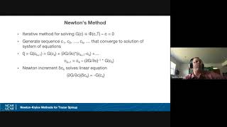
Newton's
method
is
an
iterative
method
for
solving
a
non-linear
system
of
equations
and
in
particular,
we're
applying
it
to
this.
G
function
generates
a
iterative,
so
it
generates
a
sequence
of
states
that
converge
to
the
solution
of
a
system
of
equations
and
the
way
that
it
does.
That
is
the
way
you
can
derive
Newton's
method,
I.
Think
I'm,
not
sure.
If
you
can
see
my
pointer
or
not.
A
This
is
the
expression
you
get
you're,
probably
familiar
with
this
with
one
dimensional
equations,
but
the
multi-dimensional
analog
is
just
as
written,
and
this
leads
to
a
Newton
increment
this
term
on
the
right
part
of
the
right
hand,
side
which
solves
a
system
of
linear
equations,
the
Jacobian
of
G.
With
respect
to
c
times
your
increment
equals
a
negative
of
the
right
hand,
side
the
penalty
function
for
the
current
iterate,
and
so
this
is
a
linear
system
of
equations.
A
We
want
to
solve
and
I'll
remind
you
that
this
is
a
for
the
application
that
we're
looking
at
for
just
a
single
Tracer.
This
Matrix
on
the
left
is
around
4
billion
by
4
million,
and
it
is
typically
dense.
So
it
has
many
many
non-zero
values.
This
is
not
a
matrix
that
you
can
compute
much
less
store
in
memory,
so
direct
methods
of
solving
linear
systems
of
this
solving
for
the
Newton,
increment
or
sort
of
not
feasible.
A
Minus
G,
with
the
unperturbed
initial
state
in
evaluating
G,
requires
doing
a
forward
model
run
because
that's
it
g
is
sort
of
you
plug
in
an
initial
Tracer
state
run
the
model
forward
and
G
is
end.
State
minus,
beginning
state.
So
to
compute.
This
Matrix
Vector
product
requires
a
forward
model
run
and
you
need
to
come
up
also
with
them
technique
for
selecting
the
value
of
Sigma
and
I
will
get
into
that
being
able.
A
So
this
is
how
you
can
compute
these
Matrix
Vector
products
and
there's
a
particular
class
of
iterative
methods
for
linear
systems
of
equations
that
are
well
suited
for
this
scenario,
where
you
can
compute
Matrix
Vector
products,
but
you
don't
necessarily
have
the
Matrix
itself,
let's
cry
about
iterative
methods.
This
is
why
people
call
it
Newton
cry
about
method,
so
the
crylock
methods
for
solving
linear
system
of
equations.
A
The
way
that
these
work
is
you
construct
what
is
known
as
the
a
cryolog
basis.
This
is
named
after
the
mathematician
krylov,
where
you
have
a
an
initial
vector
and
you
construct
a
basis
by
multiplying
your
vector
by
your
Matrix
repeatedly
and
up
to
a
size
of
the
Matrix
B's
will
turn
up
to
the
rank
of
the
Matrix.
These
basis,
vectors
will
be
linearly
independent
of
each
other,
and
then
you
look
for
a
linear
combination
of
base
of
vectors
from
this
basis
that
minimizes
this
residual.
A
A
You
want
P
to
be
some
sort
of
approximation
to
the
inverse
of
the
Jacobian,
but
it
would
I'd
be
ideal
if
it
were
the
inverse,
but
that's
not
practical
to
do
that,
because
we
don't
have
that
on
hand
in
it
to
be
practical,
multiplying
P,
but
it
should
be
feasible.
So
we
need
to
have
some
we're
balancing
these
two
criteria
that
somehow
is
approximating
the
inverse
of
the
Matrix
and
right
press
the
button
at
advancement.
A
It's
like
excuse
me:
we
there's
some
feasibility
to
applying
Matrix
p
particular
approach
that
we
take
to
constructing
P
was
laid
out
in
the
lead
in
Provo
paper,
so
we
take
a
sparse
approximation
to
the
Jacobian
matrix
and
it's
a
of
a
particular
form
where
we
can
compute
the
inverse
of
it
of
G
of
P.
Excuse
me-
and
this
is
based
on
the
time,
mean
induction
mixing
operators
which
have
been
extracted
from
Diagnostics
that
we
add
to
the
ocean
model.
A
To
this
system
of
equations,
and
then
we
use
the
GMS
solver
to
solve
for
the
Newton
increment
The,
Matrix,
Vector,
multiplies
and
GM
res
are
approximated
with
a
model
run,
and
we
use
a
preconditioner
based
on
a
sparse
approximation
to
the
Jacobian,
and
this
is
a
very
admittedly
high
level
description
of.
What's
going
on,
there's
numerous
technical
details
that
I'm
skipping
for
the
sake
of
time.
A
So
how
does
it
work
here?
Are
some
results
of
applying
this
to
a
buy
one
cesm
pop
configuration
from
a
normal
year,
forced
ocean
ice
configuration
to
the
ideal
age
Tracer
and
in
particular
what
I'm
looking
at
is
it's
hard-coded
in
this
in
these
results,
doing
four
cryolab
iterations
for
Newton
iteration,
which
is
quite
a
pretty
small
number,
and
that
have
a
number
of
plots
showing
convergence
properties
as
a
function
of
Newton
iteration.
A
So
this
is
looking
at
the
change
in
age.
Over
one
year
of
simulation,
the
L2
Norm
is
being
shown
in
this
panel
a
and
we're
getting
exponential
after
this
was
initialized
with
zeros.
So
it
took
a
while
for
Newton's
method
to
sort
of
kick
into
gear.
Of
one
aspect
of
the
convergence
of
Newton's
method
is
that
it
converges
super
linearly.
What
you
are
up
close
to
your
solution,
I
started
with
something
far,
so
it
sort
of
had
to
get
get
going
after
a
couple
iterations,
and
then
it
was
converging
exponentially
here.
A
That
said
where
the
RMS
globally
evaluated
RMS
after
a
handful
of
Newton
iterations
is
a
one
year
per
century
and
that's
the
RMS
is
sort
of
skewed
towards
the
grid
points
where
the
drift
is
the
highest
and
then
panel
C
I'm,
showing
a
histogram
after
five
Newton
iterations
of
the
the
change
in
ideal
age
from
end
state
to
beginning
state.
So
this
is
where,
at
five,
the
RMS
is
around
10
to
the
minus
two.
A
Where
a
lot
of
the
volume
of
the
ocean
is
seeing,
the
drift
is
around
10
to
the
minus
four
years
per
year
after
five
of
Newton
iterations
and
then
in
the
bottom
D.
This
is
showing
that
after
10
iterations,
we
see
this
sort
of
almost
normal
distribution
of
drift
in
ideal
age.
So
we're
seeing
something
like
10
to
the
minus
seven
years
per
year.
A
This
was
for
ideal
age,
which
is,
admittedly,
a
simple
tracer.
The
Newton
crime
law
solver
treats
the
boundary
condition
of
IH
as
if
it
were
just
restoring
to
a
surface.
So
there's
a
restoring
the
surface
value
to
zero
with
a
very
short
time
scale
and
there's
no
Source
seek
terms
where
there's
a
constant
Source
term
in
the
ocean
interior.
A
So
what
are
the
techniques
that
we've
been
investigating
to
apply?
The
new
crylov
solver
to
bio2
chemical
tracers
in
Marble
is
the
name
of
the
biogeochemistry
library
that
we're
using
in
cesm
and
Mike
is
going
to
talk
about
the
reporting
of
Marvel
coupling
of
marble
to
Mom
six
one
aspect
of
these
advisory
chemistry.
Chasers
is
the
ecosystem
variables.
That's
just
like
the
python
themselves.
The
tracers
have
very
non-linear
behavior
on
time
scales.
Much
shorter
than
the
time
skills
that
the
Newton
cry,
lab
solver
is
integrating
over
is
sort
of.
A
A
So
what
are
the
approaches
that
we're
using
is
to
do
a
short
run
where
you
spin
up
the
biological
pump
then
apply
the
Newton
cry,
love
to
spin
up
nutrient
fields,
which
aren't
quite
so
non-linear
and
have
longer
time
scales
Dynamics
with
the
biological
Pub
prescribed
from
Step
One,
and
then
repeat,
so
you
spit
up
nutrients
with
a
fixed
prescribed
biological
up
and
then
do
a
short
run
to
update
the
nutrients.
Then
re-spin
up
the
biological
pump
with
these
updated
spun
up
nutrients
and
go
through
this
Loop.
A
Source
sync
terms
from
the
real
tracers
and
we
are
applying
the
Newton
cry,
love
method
to
the
shadow
tracers
in
the
shadow
tracers
do
not
feed
back
to
the
biological
pump.
So
by
doing
this,
the
the
bottle
is
simulating
with
each
iteration
of
the
root
and
cryov
Method.
It's
re-stimulating
the
same
biological
Pub,
but
the
increments
that
are
in
the
method
that
are
being
applied
are
being
applied
only
to
the
shadow
nutrients
in
this
sort
of
avoids
these
short
time
scale,
not
only
linearities.
A
A
In
the
current
version
of
the
solver
Newton
cry
about
software
that
it's
been
developed,
it
can
be
applied
not
only
to
tracers
and
gcms,
but
it
can
be
applied
to
it's
been
developed
now
at
a
sort
of
abstract
way.
So
you
can
apply
it
to
something
like
a
1D
phosphorus
model.
That
of
any
sort
of
model
doesn't
have
to
be
a
full-blown
GCM,
and
this
allows
for
experimenting
with
different
solver
developments
and
a
simple
model,
and
that
could
run
these
now
on
my
laptop.
A
A
So
while
we
were
getting
convergence
with
this
restoring
strategy,
the
convergence
is
much
slower
than
what
we
see
for
a
simple
Tracer
like
ideal
age.
So
another
approach
that
we
tried
is
a
mimicking
biological
uptake
on
the
shadow
tracers,
so
they
restore
the
shadow
Tracer
to
the
real
tracer,
with
a
rate
that
mimics
biological
uptake
to
take
the
derivative
of
phosphate
uptake
with
respect
to
phosphate,
and
this
gives
you
a
whatever
time
scale.
A
So
moving
forward
applying
this
to
our
full-blown
carbon
cycle
model
ecosystem
model
of
we're
going
to
be
looking
at
where
sophisticated
of
restoring
techniques
just
expect,
because,
based
on
this
experience
in
our
1D
model,
so
some
ongoing
work
with
applying
this.
This
projects
of
the
Newton
dialogue
solver
on
Ocean
tracers,
is
still
very
much
a
work
in
progress
and
some
open
questions
and
projects
that
are
going
on
are
dealing
with
intra-annual
variability
of
circulation.
A
A
first
order
question
is:
is
it
appropriate
to
be
seeking?
If
you
have
a
non-cycle
stationary
circulation,
is
it
appropriate
to
end
State
equals
your
beginning
state?
Where
that's
not
the
case
say
for
your
temperature
Fields,
the
Newton
cryov
solver
will
happily
generate
a
solution
but
interpret
interpreting.
That
solution
is
a
little
bit
complicated
when
the
circulation
is
itself
non-cyclos
stationary-
and
this
also
applies
to
when
you
have
internally
generated
variability
in
a
for
instance.
A
A
I
have
to
admit,
though,
the
appropriate.
Restoring
formulation
is
not
exactly
obvious
how
to
do
that.
I
haven't
really
talked
much
about
mom,
so
we
are
investigating.
This
is
a
bomb
six
webinar,
so
we
are
investigating
the
work
in
progress
to
apply
the
Newton
cry
about
solver,
to
Mom,
six
and
initially
within
the
context
of
cesm,
where
I
have
the
scripting
framework
for
doing
model
runs
already
at
the
end
and
there's
some
challenges
to
this
already
and
I've
had
some
valuable
conversations
with
Andrew
Chow
that
address
some
of
these.
B
A
Can
just
take
a
grid
Point
by
this
grid.
Point
value
minus
another
three
point
value
because
they
correspond
to
the
same
physical
space,
but
that
is
not
the
case
when
you
have
a
time
varying
vertical
coordinate
and
the
initial
approach
that
we're
we're
going
to
be
trying
to
do
is
evaluate
both
sides
with
a
fixed
depth
or
Z
Star
coordinate
so
initialize.
The
bottle
with
Tracer
State
on
a
d
coordinate
and
then
spit
out
on
the
same
depth.
A
The
same
fixed
depth,
coordinate
to
compute
the
dirt
the
differences
and
then
up
the
Jacobian
will
be
defined
with
respect
to
model
output
on
that
same
depth,
coordinate,
there's
some
complications
of
handling
the
tripod
C
and
getting
appropriate
diagnostics
for
the
preconditioner
Andrews
neutral
density
mixing
scheme
has
some
complications
by
introducing
more
coupling
between
adjacent
grid
points
in
different
parts
of
the
column,
so
a
naive
implementation.
They
need
to
significant
fill
in
in
solving
the
preconditioner
equations,
which
then
has
a
big
increase
in
the
amount
of
memory
which
can
be
problematic.
A
C
D
A
D
B
Thanks
for
the
talk
I
had
a
question
about,
is
there
could?
Is
there
a
physical
interpretation
to
the
Newton
iteration
in
this
method?
Like?
Is
there
anything
useful
that
we
can
kind
of
gain
out
of
it
any
kind
of
insights?
Or
is
it
really
just
the
end
state
of
it
is
the
the
most
important
part
of
it.
A
I
I'd
have
to
think
through
about
the
Jacobian
to
apply
inverted,
the
Jacobian
against
the
penalty
function
if
I
think
of
the
1D
examples
of
Newton's
methods,
you're
looking
at
a
tangent
line
and
extrapolating
that
tangent
line
to
zero-
and
this
is
something
analogous
to
that.
But
I
don't
see
how
to
interpret
that
say
in
terms
of
ocean
circulation
in
the
high
dimensional
context.
E
Oh
yeah
I
had
a
question,
so
you
mentioned
this
question
of
how
long
is
necessary.
For
instance,
in
the
presence
of
inter-annual
non-cycle
stationary
variability
to
sort
of
get
a
representative
circulation.
I
was
wondering
to
what
extent
that
can
or
even
is
I
guess
decoupled
from
non-stakel
stationarity
in
the
Tracer
boundary
conditions
that
could
be
imposed
at
the
ocean
domain.
Is
that
sort
of
built
into
the
Newton
cry
love
or?
Is
that
separate.
A
C
F
F
A
Then
re-initialize
the
real
temperature
and
salinity
from
the
spun
up
temperature
and
salinity
and
then
do
a
short
integration
of
the
Velocity
Fields
with
the
incremented
temperature
and
salinity
wow.
So
this
is
either
the
reason
why
I
have
some
optimism.
Optimism
that
this
might
work
is
that
with
the
biology,
the
idea
going
on
is
that
the
ecosystem
spins
up
relatively
quickly
to
the
nutrient
fields
in
the
analogy
is
I'm.
G
Thanks
Keith,
that
was
a
really
nice
talk.
One
question
that
kind
of
comes
to
mind.
As
you
talk
about
the
challenges
with
non-stationarity
and
dealing
with
non-linearity
is
whether
there
are
things
that
could
be
drawn
from
the
control
theory,
literature
that
might
be
combined
here
it
with
control
theory,
it's
kind
of
a
way
of
doing
data
assimilation,
if
you
want
to
think
of
it
that
way,
but
it's
it's
really
putting
in
kind
of
artificial
terms
that
that
drive
things
towards
the
desired
State,
and
it's
it's
very
well
established.
G
A
lot
of
the
literature
is
so
old
that
it's
not
really
in
the
engineering
literature.
The
the
story
is
that
when
it
was
first
introduced,
this
was
in
coal-fired
battleships
and
it
caused
the
bridge
Crews
to
Revolt,
because
it
did
too
good
a
job
of
scaring
better
than
than
the
guy
with
his
hand.
So
a
lot
of
it
dates
back
to
the
19th
century,
so
Wikipedia
is
actually
a
good
place
to
start
or
kind
of
textbooks.
It's
it's
old
stuff.