►
From YouTube: 3rd PAWS Webinar
Description
The third webinar from the Paleoclimate Advances Webinar Series (PAWS) which took place on May 6th 2022.
Dr. Dan Lunt discussed "(Paleo)climate sensitivity in the IPCC" and Martin Renoult discussed "Constraining climate sensitivity from paleoclimate temperatures: Robust or weak approach?"
For more information and to signup for the PAWS Google Group visit:
https://www.cesm.ucar.edu/events/webinars/paws/
A
B
All
right
can
people
see
my
screen
and
hopefully
hear
me
all
right.
So
let's
go
ahead
and
get
started
thanks.
Everyone.
Thank
you
all
for
joining
us
for
our
third
paleoclimate
advances,
webinar
series
or
pause
for
short,
I'm
clay,
tabor
I'll
help
out
with
hosting
today.
Before
we
get
into
the
talks.
I
just
have
a
few
reminders
about
our
values
and
our
format.
B
So
the
goals
of
paul's
is
to
provide
a
welcoming
space
for
the
exchange
of
ideas
on
paleoclimate
advances,
so
please
make
sure
to
be
respectful
and
supportive
of
each
other,
especially
during
the
question
and
answer
in
the
discussion.
Also,
please
remember
to
consider
nominating
people
for
future
speakers.
Remember.
We
strongly
encourage
self
nominations
as
well,
so
our
format's
the
same
as
in
the
past
few
times,
we'll
start
out
with
20
minutes
for
talks
I'll.
B
Let
the
speakers
know
when
we
have
two
minutes
remaining
and
after
each
talk
there
will
be
about
five
minutes
for
question
and
answer.
So
please
save
your
questions
for
the
end
of
the
talks
and
raise
your
hand
at
that
time
or
post
them
in
the
chat
and
after
we've
had
both
talks
completed
with
those
five
minutes
for
question
answers,
then
we'll
have
an
additional
10
minutes
for
more
general
discussion
and
these
talks
are
being
recorded
and
will
be
posted
online
as
well
all
right.
So
we
have
two
exciting
talks
today
on
paleoclimate
and
climate
sensitivity.
B
Our
first
speaker
is
dan
lund.
Dana
is
a
professor
of
climate
science
at
the
university
of
bristol
his
research
centers
on
past
climate
change,
with
a
focus
on
understanding
how
and
why
climate
has
changed
in
the
past
and
what
we
can
learn
about
future
from
the
past
he's
a
lead
author
on
the
ipcc
assessment
report
and
he
leads
the
international
deep
mip
program.
B
He
was
also
founding
and
chief
executive
editor
of
the
journal
of
geoscientific
model
development
and
is
an
affiliate
at
science
affiliate
scientist
at
incar.
Our
second
speaker
is
martin.
Renew
martin
is
a
phd
candidate.
Currently
at
stockholm
university
he
studies,
paleoclimate,
modeling
and
reconstructions,
and
what
we
can
learn
about
climate
dynamics
from
paleoclimates.
B
C
I'll
just
share
my
screen
hope
you
guys
can
see
those
slides
now
yeah,
so
I'm
gonna
really
well.
First
of
all,
I'm
very
briefly:
gonna
just
introduce
the
chapter,
seven,
which
was
the
chaps
I
was
involved
in
in
the
most
recent
ipcc
report
and
then
for
most
of
the
talk
I'll
focus
on
climate
sensitivity
and,
in
particular
the
paleoclimate
sensitivity
assessment
that
we
carried
out
as
part
of
as
part
of
ar6,
so
but
just
to
kick
off
as
a
very
brief
intro.
C
This
is
our
chapter
chapter:
seven,
the
earth's
energy
budget,
climate
feedback
and
climate
sensitivity,
so
just
to
give
a
bit
more
of
a
broad
overview
of
the
whole
chapter
and
the
things
that
are
covered
in
there.
I
think
these
new
elements
it
talks
about
down
here
is
quite
useful.
So,
basically
a
lot.
C
Both
you
know
spatially
and
different
heights,
and
what
have
you
to
assess
an
overall
cloud
feedback,
a
lot
of
work
on
on
the
pattern
effect
and
how
that
how
we
understand
recent
historical
changes
in
terms
of
patterns
of
sea,
surface
temperature
change
and
then
the
bit
I'm
going
to
focus
on.
Is
this
new
assessment
of
climate
sensitivity?
C
And
then,
finally,
there
was
a
section
also
looking
at
quantifying
some
of
these
key
metrics
that
are
used
by
policymakers
to
link
emissions
of
co2
and
and
methane
to
to
temperature
targets.
So
that's
sort
of
an
overview
of
the
chapter
like
I
said,
I'm
going
to
focus
on
myself
on
on
climate
sensitivity
in
the
in
the
sixth
assessment
report,
and
in
particular
you
know,
I
guess
the
first
thing
to
say
is
even
the
definition
of
climate
sensitivity
changed
a
little
bit
in
this
report.
C
In
that
you
know,
we
think
about
the
global
mean
global
mean
annual,
mean
temperature
equilibrium,
temperature
response
to
a
doubling
of
atmospheric
co2.
But
a
new
thing
in
this
report
was
that
we
made
it
very,
very
clear
that
this
was
actually
including
all
feedbacks
in
the
climate
system,
apart
from
those
associated
with
ice
sheets
and
those
associated
with
co2
itself.
So
in
in
previous
reports,
it
was
more
done
on
sort
of
the
time
scale
of
the
feedbacks,
but
this
time
it
was
a
more
sort
of
physically
based
physically
based
definition.
C
Just
very
briefly,
I'm
sure
all
of
you
know
this,
but
you
know
climate
sensitivity.
Ecs
is
a
key
metric
because
it
allows
us
to
make
a
link
basically
between
co2
concentrations
and
temperature.
So,
for
example,
if
you
have
a
key
temperature
target
like
one
and
a
half
degrees
warming,
it
allows
you.
It
basically
tells
you
what
equilibrium
co2
concentration
is
is
consistent
with
that.
C
So
before
ar6,
this
was
the
situation,
how
climate,
how
ecs
climate
sensitivity,
how
different
key
assessments,
mainly
from
the
ipcc
here
from
the
first
assessment
or
to
the
fifth
assessment
report,
how
that
assessment
had
changed
and
you
can
see
the
key
thing
as
everyone
knows,
is
that
really
the
overall
assessment
of
the
likely
range
of
climate
sensitivity
had
not
really
changed
since
the
mid
70s
since
the
first
chinese
report,
so
it
was
really
interesting
starting
work
on
this
chapter
to
think.
Well,
can
we
go?
Can
we
go
beyond
that?
C
Are
we
about
to
tighten
these
constraints
or
not,
maybe
they're
even
going
to
widen,
like
they
did
between
ar4
and
ar5?
With
you
know,
it's
improved
understanding
doesn't
always
lead
to
narrower
estimates.
It
can
actually,
if
you
improved
understanding,
can
mean
actually
your
uncertainty
gets
larger,
and
so
this
time
around,
we
have
four
lines
of
evidence
to
base
our
assessment
on
process-based
estimates
and
I'll
go
through
these
briefly
process.
Best
estimate
the
historical
record,
paleo
climates
and
emerging
constraints.
C
So,
first
of
all,
the
first
of
these
process
based
assessment
of
climate
sensitivity.
This
is
basically
trying
to
assess
the
magnitude
of
all
the
feedbacks
that
you
can
think
of
in
the
climate
system
and
then,
basically
adding
them
together,
defining
them
with
a
with
a
feedback
parameter
with
units
of
watts
per
meter,
squared
per
kelvin
and
then
basically
adding
them
all
together
to
get
an
overall
feedback
parameter.
So
key.
C
Feedbacks
and
some
of
the
input
to
this
was
the
cmip6
models
themselves,
which
can
be
used
to
estimate
some
of
the
sort
of
basic
feedbacks
like
the
planck
feedback,
wood,
vapor
and
lapse
rate
feedback
service.
Albedo,
like
I
said
here,
we've
got
the
large
uncertainty
in
the
cloud
feedbacks,
but
also
this
time
around.
C
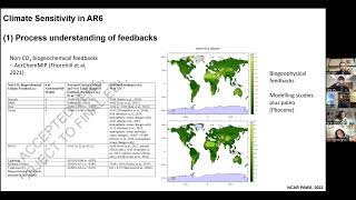
This
was
an
element.
This
was
a
part
where
paleoclimate
played
a
role,
so
in
particular
here.
What
we're
talking
about
really
is
the
albedo
feedback
associated
with
vegetation
changes
in
response
to
temperature
change,
and
you
know
there
are
a
few
modeling
studies
that
have
looked
to
this,
where,
for
example,
people
run
models
into
the
future
with
and
without
vegetation
feedbacks,
but
in
terms
of
observational
lines
of
evidence,
because
it's
quite
a
long
time
scale.
C
Feedback
and
the
paleoclimate
can
provide
some
data
for
this,
and
in
this
case
we
used
the
pliocene,
the
midply
scene
three
million
years
ago.
There's
a
line
of
evidence
here
because
there's
pollen
data
that
tells
us
something
about
how
vegetation
types
were
different
in
the
plot
in
the
pliocene
when
co2
was
high,
temperature
was
high
and
we
were
about
to
be
able
to
make.
We
were
able
to
make
a
sort
of
first
order,
estimate
of
the
feedback
parameter
associated
with
that
vegetation
feedback
from
observation
from
paleo
observations
and.
C
That
it
was
actually
quite
a
bit
larger
in
magnitude
than
the
estimates
that
we
get
from
from
many
models,
so
that
was
one
the
first.
The
first
example
I
have
really
a
paleoclimate
coming
into
the
overall
assessment
of
climate
sensitivity
through
characterizing
the
size
of
vegetation,
feedbacks,
but
also
another
another
part
of
this
chapter
was
was
looking
at
the
non-linearity
of
some
of
these
feedbacks
and
how
they
vary
themselves
as
a
function
of
temperature,
because
that
can
be
important
for
assessing.
C
But
if
the
feedback
is
very
non-linearly,
then
maybe
that's
a
poor
assumption,
and
this
is
again
is
something
where
paleoclimate
can
have
something
to
say
about
this.
If
you
can
estimate
temperature
and
co2
changes
across
a
range
of
different
states
like
we
did
in
like
people
have
done
looking
at,
for
example,
the
early
year
scene
compared
to
the
late
earth
scene
compared
to
the
fire
scene
or
looking
at
feedbacks
at
the
lgm
compared
to
the
present
day,
then
you
can
get
a
feeling
for
this.
C
For
the
magnitude
of
this
non-linearity
and
there's
again
a
few
modeling
studies
that
have
done
this
either
under
modern
or
paleo
conditions
and
observational
studies
again
from
you
know,
pure
paleo
data,
and
we
put
all
these
together
on
this
on
this
graph,
which
shows
the
feedback
parameter
strength
on
the
y-axis.
So
you
basically
got
increasing
climate
sensitivity
as
you
go
up
here
as
a
function
of
background
temperature.
You
can
see
these
are
quaternary
records,
looking
at
climate
sensitivity
in
the
lgm
compared
to
the
modern
and
then
you've
got
some
other
paleo
records.
C
So
how
sort
of
the
strength
of
that
nonlinearity?
So
obviously,
still
a
lot
of
you
know
a
lot
of
work
that
could
be
done
from
the
purely
from
the
paleo
data
side.
Here
the
second
line
of
evidence
was
looking
at
the
instrumental
record
the
last
150
years,
or
so
you
know
what
the
various
different
forcings
are,
of
course,
that
temperature
chain
you've
got
an
estimate
of
the
temperature
change
itself.
C
Then
you
can
estimate
the
climate
sensitivity
if
you
take
into
account
some
of
the,
and
this
is
again
something
sort
of
new
in
this
report
compared
to
the
previous
report.
If
you
take
into
account
the
fact
that
some
of
the
sort
of
the
lags
the
time
scale
of
response
of
the
climate
system
and
how
feedbacks
change
as
this
as
the
patterns
of
sea
surface
temperature
change
are
evolving
in
response
to
the
co2
force.
C
C
C
You
know
with
a
given
uncertainty
associated
with
the
uncertainty
in
the
calibration,
the
proxies
and
the
uncertainty
in
going
from
individual
records
to
a
global
mean
as
long
as
you
take
into
account
all
those
uncertainties
and
take
into
account
the
forcing
effect
of
the
ice
sheets,
which
is
not
itself
included
in
the
climate
sensitivity.
If
you
sort
of
take
that
out
of
the
forcing
and
the
response.
C
Then
it
allows
you
to
estimate
the
climate
sensitivity
and
basically
to
assess
the
climate
sensitivity
from
these
various
different
lines
of
evidence.
We
basically
accumulated
all
the
studies
that
we
have
had
since
ar5
and
sort
of
tabulated
them,
along
with
their
estimate
of
ecs
and
their
uncertainty.
C
You
know
there
are
several
pages
in
the
report
outlining
the
details
of
this
assessment,
but
just
very
much.
In
summary,
we
went
for
a
sort
of
quite
a
qualitative
approach,
really
taking
into
account
looking
at
these
different
studies
to
come
up
with
a
you
know.
Eventually,
we
have
to
come
up
with
a
quantitative
estimate,
but
our
our
approach,
our
methodology,
was
to
really.
C
E
C
A
E
C
Very
likely
that
ecs
was
greater
than
1.5
purely
from
the
paleoclimate
evidence.
We
were
asked
also
to
come
up
with
a
best
estimate
and
again
there's
very.
There
are
lots
of
different
ways
of
doing
this
sort
of
to
get
a
central
estimate.
But
you
know
we
did
several
different
methods
and
they
all
came
up
with
a
similar
answer.
C
So,
for
example,
if
you
just
very
simply
take
an
average
of
the
well
for
the
first
thing
we
decided
to
do
is
actually
take
out
those
studies
that
came
from
the
transient
records
of
the
quaternary,
because
you've
got
lots
of
complications
associated
with
how
much
of
the
response
is
associated
with
ice
sheets.
How
much
of
it
is
associated
with
direct
orbital,
forcing
and
also
yeah,
so,
basically
mainly
due
to
the
complications
of
the
orbital
signal.
That's
in
there.
C
If
you
take
those
ones
out,
and
then
you
average
separately
over
all
the
lgm
studies
and
the
pre-quaternary
studies,
then
basically
you
get
an
estimate
of
something
like
just
over
three
degrees
c.
So
our
best
estimate
was
somewhere
between
three
and
well
three
point
three
and
three
point:
four
again:
if
you
didn't
look
at
the
pre
quaternary,
if
you
took
out
the
preterite
studies,
then
if
you
look
at
the
upper
range
now
of
previous
work,
the
lgm
the
highest
value
was
4.4.
C
If
you
look
at
the
pre-quaternary,
the
highest
was
4.9,
but
take
into
account
the
state
dependence.
The
fact
that
we
think
planet
sensitivity
increases
with
increasing
temperature.
We
said
it
was
likely
that
ecs
was
less
than
4.5.
Just
a
reminder.
The
language
for
the
language,
that's
very
likely,
is
a
90
confidence.
The
likely
is
a
two-thirds
two-thirds
confidence.
C
And
then
also
we
looked
again
if
you
exclude
those
pre-quaternary
studies,
the
evidence
that
it
was
extremely
unlikely-
which
I
think
is
the
95
percent
confidence
that
the
ecs
was
below
8
degrees.
So
that
was
our
overall
assessment
from
the
paleo
data
that
third
line
in
terms
of
the
fourth
line
of
evidence.
That
was
from
emerging
constraints,
but
I'm
not
even
going
to
mention
these
at
all,
because
I'm
sure
martin
will
give
us
a
very
good
nice
introduction
to
those.
C
C
C
You
basically,
because
you
exclude
more
high
climate
sensitivity
models,
then
you
exclude
low
climate
sensitivity
models
by
doing
this,
and
you
end
up
with
an
overall
decrease
in
temperature,
and
I
you
know
what
I
always
say
is
basically
because
the
paleo
climate
data
was
one
of
the
lines
of
evidence
that
we
used
in
that
assessment,
then,
basically,
the
paleoclimate
data
has
effectively
brought
down
these
projections
of
the
future.
In
the
ipcc
report,.
C
C
We've
got
the
the
historical
record
so,
like
you
know,
roughly
1850
to
the
recent
we've
got
potential
1970s
to
today.
Here
we've
got
the
last
glacial
maximum
mid-pricing
warm
period
the
earliest
in
and
for
all
of
these
we've
got
the
global
mean
temperature
relative
to
pre-industrial.
Basically,
so,
for
example,
this
shows
that
and
in
the
black
squares
we've
got
the
black
circles
and
their
own
uncertainty.
We
basically
got
the
observations
in
this
case.
This
is
sort
of
historical
observations
of
warming
since
1850
here
we've
got
about
about
one
degrees,
c
or
so.
C
Warming
since
1975
about
0.5
degree
in
observations,
eco
warming,
for
example,
about
15
degrees
compared
to
pre-industrial
what
the
circles
are
showing.
You
are
gcm
estimates
of
that
same
observed
warming,
so
each
circle
is
a
different,
the
different
gtm.
These
are
all
cnip
six
models
for
the
historical
and
post
1975..
C
Once
you
get
out
to
the
eco,
you
know.
None
of
these
are
marks.
You
know.
One
of
these
is
the
siemens.
Two
of
these
are
siemens
six
models,
but
you
know
fewer
and
fewer
cmx-6
models
once
you
get
to
the
paleo
simulations,
those
that
are
red
and
blue
are
basically
gcms
or
esm
that
have
a
climate
sensitivity
that
is
outside
the
range
of
our
assessed
climate
sensitivity,
so
the
red
ones
have
an
ecs
greater
than
five,
and
the
blue
ones
have
an
ecs
less
than
two
and
what
it
shows,
I
think
very
nicely
is.
C
F
C
C
So
again,
those
feedbacks
are
included
in
the
observations
and
in
the
response
when
it
comes
to
the
lgm
again,
the
paleo,
the
paleo
observations
themselves
include
those
feedbacks,
but
my
understanding
is
that
most
of
these
gcns
had
fixed
vegetation,
although
I'm
not
sure
about
that
some
of
them
one
or
two
of
them
might
be
including
vegetation
feedbacks.
But
my
understanding
is
a
lot
of
these
actually
had
fixed
vegetation,
and
so
it
didn't
didn't
actually
include
that
effect.
C
I
was
just
going
to
say
when
it
comes
to
the
cmip6
models.
It's
you
know
it's,
I
don't
I
don't
know
actually
which
of
these
did
and
which
of
these
didn't
include
vegetation
feedbacks.
If
you
take,
for
example,
the
uk
model,
there
are
two.
There
are
two
different
versions
of
the
uk
model
in
here
which
had
gem
3,
which
doesn't
include
those
feedbacks
in
uk
esm,
which
I
believe
does
include
those.
So
it's
variable
between
models.
Once
you
get
to
the
historical
record.
C
So
in
terms
of
the
cons,
well,
I
get,
I
think
they
are.
I
think
the
answer
to
that
is
yes,
because
when
we
assess
climate
sensitivity,
one
of
the
feedbacks
that
we
included
was
the
biophysical
vegetation
feedback
and,
in
fact,
the
way
that
we
assessed
that
was
through
paleo
observations
of
vegetation
change.
F
B
Maybe
we
can
pick
this
up
in
the
discussion
at
the
end
yeah.
So
for
the
sake
of
time,
we
can
wrap
back
around
to
this
now
so
there's
a
question
in
the
chat
from
jack,
but
we
can
talk
about
these
further
in
the
discussion,
but
we
can
go
ahead
and
jump
into
martinstock
again
20
minutes
I'll.
Try
to
give
you
a
two
minute
warning
and
then
five
minutes
for
questions
on
this
and
then
I
think
we
can
come
back
and
circle
back
around
to
these
questions.
G
G
G
That
here
are
represented
as
blue
dots,
so
that
you
can
build
like
a
real
statistical
relationship
which
is
going
to
be
the
red
line
here
and
then
the
idea
is
that
you're
going
to
use
this
red
relationship
by
putting
a
geological
reconstruction
of
the
temperature
of
those
aloe
climates,
so
a
temperature
that
exists
in
the
real
climate
system.
So
you
can
infer
the
real
value
of
climate
sensitivity
and
so,
as
I
said
before,
you
can
just
write
it
as
simple.
As
s
is
equal
to
some
regression
parameters
times
the
paleoclimate
temperatures.
G
And
so
the
the
way
you
do
it
is.
Basically,
you
only
need
an
ensemble
of
climate
models
that
are
going
to
simulate
the
same
past
climate,
and
so
thanks.
We
have
the
paleoclimate
modeling
intercomparison
project,
which
designed
those
paleo
simulations
with
similar
boundary
conditions
across
different
generations
of
modeling,
and
so
you
can
use
this
ensemble
of
models
in
emerging
constraint
framework
and
so
in
the
latest
super
four.
G
G
G
Ideally,
you
also
want
the
largest
signal-to-noise
ratio,
which
means
that
you
would
like
to
avoid
paleoclimate
that
are
not
so
different
from
pre-industrial
temperatures,
and
the
last
point
is
actually
very
interesting,
but
it's
very
specific.
You
actually
need
to
know
the
value
of
climate
activity
of
the
models
you
are
using,
and
this
is
mostly
a
problem
for
models
of
pineapple
one.
G
G
And
so,
if
we
follow
those
four
points,
basically,
we
can
exclude
already
the
last
integration
and
the
immediate
holocene
to
constrain
climate
centrity,
just
because
they
have
quite
a
low
signal
to
noise
ratio.
The
temperature
are
quite
close
of
pre-industrial,
so
they're
not
ideal
candidates,
particularly
compared
to
the
glycine
and
a
lot
of
special
maximum,
which
are
much
have
much
stronger
temperature
signals.
G
So,
just
to
briefly
summarize
about
the
last
question
maximum
and
the
five
scenes
so
the
last
question
maximum
is,
of
course,
this
the
this
part
of
the
last
ice
age,
where
the
extent
of
the
ice
sheet
was
maximum.
So
particularly,
you
had
a
big
ice
sheet
on
north
america
and
europe
and
in
terms
of
geological
data,
because
it's
quite
close
to
us
geologically
speaking,
we
have
quite
an
advance
on
sociological
data.
G
So
on
the
right
here
is
the
temperature
reconstruction.
That
is
quite
recent.
It's
from
2022
by
ananital,
where
you
can
see
that
all
those
like
colorful
dots
are
geological,
geologically,
reconstructed,
temperature
data,
you
can
actually
use,
and
then,
by
using
this
kind
of
statistical
filtering
method,
you
can
build
those
like
global
non-special,
maximum
temperature,
reconstructions.
G
So
here
is
an
example
of
the
model
c
surface
temperature
at
the
last
question,
maximum
with
the
climate
sensitivity
of
models
during
pima,
2
and
premier
3,
and
you
can
see
that
correlation
does
not
look
so
good.
There
is
basically
limited
significant
negative
correlation
patterns
in
the
tropic,
which
is
what
you
expect.
It
means
that
the
higher
the
climate
activity
of
the
models
are
the
more
cold
they
get,
but
there
is
also
this
like
weird,
very
strong,
positive
pattern
in
the
southern
ocean,
which
is
unexpected
and
it's
going
to
bias
your
results.
G
And
so
then
the
idea
is
that,
once
you
have
your
ensemble
of
models,
you
just
take
the
com,
you
just
compute
the
temperatures
you
want.
You
can
focus
on
just
tropical
temperatures
or
global
temperatures,
and
then
you
put
them
in
this
kind
of
scatter
plot
with
climate
change,
and
then
you
build
your
emerging
relationship,
and
so
this
is
what
we
did
in
2020.
G
G
So
I
I'm
not
going
to
go
into
details
into
this
method.
What
is
important
to
to
look
at
here
is
that
for
the
case
of
the
lgm,
the
the
final
estimate
of
climate
sensitivity,
which
is
this
purple
arrow
you
can
see
on
the
x-axis-
is
actually
larger
than
the
estimate
you
will
get
from
price
in
temperature.
G
Despite
the
fact
that
the
observed
back
then
in
2020
before
the
device
was
much
much
more
certain
and
one
of
the
reason
is,
you
can
see
that
that
again,
the
quality
of
the
correlation
at
the
lgm
is
just
not
good.
Models
are
going
like
in
every
direction
and
they
don't
seem
to
really
agree
between
each
other.
On
what
they're
doing,
despite
agreeing
quite
well
with
what
the
reconstruction
is
telling.
G
Us
so
to
summarize
so
far,
I
show
you
that
we,
we
can
effectively
use
paleoclimate
temperature
in
emerging
constrained
framework
to
constrain
climate
cbt.
But
if
you
look
on
the
ideal
constraint,
it
seems
quite
weak
if
you
have
an
estimate
of
climate
censivity,
the
upper
bound,
at
least
that
easily
exceed
5.5
kelvin,
even
6
kelvin
in
the
worst
cases
and,
on
the
contrary,
the
emergency
constraint
that
come
from
blyson
temperature
seems
very
robust
and
it's
actually
getting
better
and
better
as
climate
models
are
simulating
the
lg
that
applies.
G
So
the
fact
that
the
relationship
between
lg
and
temperature
and
ecs
is
bad
is
was
not.
It
has
not
been
the
case
like
all
the
time.
So
back,
then
in
2012,
when
hargris
at
al
looked
only
at
the
pimp
to
ensemble
and
so
the
pimp
to
lgm
temperature
versus
ecs.
The
correlation
was
actually
much
better
and
it
was
just
extended
on
almost
all
the
tropic,
but
there
was
still
this
like
weird
positive
pattern.
G
Because,
first
of
all,
there
are
not
that
many
models
that
implemented
dynamical
vegetation
in
pb3
and
then,
if
you
actually
do
statistics-
and
if
you
look
at
if
those
ensembles
are
actually
statistically
different,
they
are
not
they
statistically,
they
are
almost
all
the
same.
The
median
do
not
differ
really,
it's
really
difficult
to
say
that
this
is
the
reason
why
the
correlation
looks
so
bad,
and
so,
instead
we
looked
at
different
issues
regarding
the
climate
of
the
land
special
maximum
and
we
try
to
categorize
to
see
issues
into
structural
issues
and
state
dependent
issues.
G
And
then,
when
we
talk
about
state
dependent
issues,
we
talk
about
issues
that
arise
from
differences
in
climate
dynamics
that
come
from
comparing
warm
climate
and
coal
climate,
and
here
the
main
problem
is
that
climate
sensitivity,
as
it
is
currently
is
being
mostly
diagnosed
from
warm
simulation.
So,
typically,
you
do
four
times
to
simulation,
and
then
you
try
to
compare
that
to
the
cold
temperature
of
the
lgm,
where
climate
feedbacks
probably
behave
in
a
different
way,
as
it
has
been
also
shown
now
in
the
ipcc.
G
This
is
interesting
because
these
results
actually
change
drastically
across
climate
models.
This
is
something
we
got
from
mpi
esm
1.2,
but
you
will.
You
could
see
that
in
some
other
models,
notably
miroc,
actually
the
lgm
boundary
conditions
impact
much
more.
The
changes
in
cloud
feedback
than
halving
or
doubling
concentrations
of
co2.
G
Finally,
another
problem
is
at
the
time
of
the
research
and
really
emphasizing
on
this.
At
a
time
of
the
research,
there
was
only
a
single
model
that
has
a
high
climate
sensitivity,
so
climate
center,
both
five
which
was
csm2,
and
it's
a
bit
of
a
problem
for
the
lgm.
As
I
said
at
the
beginning,
because,
basically,
if
you
include
csm2,
you
will
end
up
with
a
correlation
map
which
is
on
the
top.
But
then,
as
soon
as
you
exclude
csm2,
you
will
have
the
correlation
map,
which
is
at
the
bottom.
G
And
so
now
to
talk
more
briefly
about
the
pliocene,
because
this
is
quite
ongoing
and
future
work.
So
for
the
appliances
there
there
are
not
that
many
issues
actually,
as
I
said
at
the
beginning,
correlation
map
looks
really
good
and
the
biggest
concern
back
then
was
the
very
large
uncertainty
we
had
on
the
geological
reconstruct
reconstruction.
G
So
one
of
the
question,
of
course
you
can
ask
yourself-
is
that:
is
it
actually
too
good
to
be
true?
So
on
the
right
is
a
map
of
the
data
of
the
pricing
we
have
that
is
currently
used
in
pmb4
and
you
can
see.
As
I
said
at
the
beginning,
there
is
quite
a
scarcity
of
data
in
the
polar
oceans,
particularly
in
the
southern
ocean.
So
there
might
be
that
estimate
you
can
get
from
place
in
temperature
will
be
really
heavily
biased
by
the
reconstructions
you
actually
provide.
G
Something
good,
though,
that
exists
in
clients
and
simulation
is
this
abundance
of
sensitivity,
experiments.
They
have
a
lot
of
sensitivity,
experiment
when
they
interchange
the
eye
sheet
of
the
pliocene
or
the
vegetation
or
co2,
and
so
we
could
learn
how
sensitive
the
relationship
between
price
and
temperature
ecs
is
to
those
changes,
something
that
will
be
ideal
with
the
lgm
to
really
pin
down
what
is
the
contribution
of
ice
sheet
forcing
and
finally,
of
course,
you
could
combine
this
kind
of
very
strong
estimate
with
the
historical
emerging
constraint
to
have
an
even
better
estimate.
G
So
the
last
question
maximum
is
widely
simulated,
but
it
seems
to
be
quite
a
weak
emerging
constraint,
incline,
accessibility,
models
and
sensitivity.
Experiments
could
either
improve
that
constraint
or
just
give
us
information
on.
Why
is
it
so
bad,
and
so
finally,
the
pleisin
is
clearly
the
most
obvious
constraint
today,
but
there
might
be
some
large
uncertainties
that
are
neglected.
B
C
Thanks
thanks,
martin,
a
really
nice
really
nice
talk.
I
guess
just
to
comment
on
the
comment
on
the
pliers
here.
You
mentioned
the
uncertainties
in
the
the
temperature
reconstructions,
meaning
you
know
we're
not
quite
sure
you
know
where
we
should
be
on
the
on
the
y-axis.
I
guess
of
your
plot
of
your
plot,
but
also
the
bigger
major
uncertainty
using
the
pliocene
for
emerging
constraints.
C
Is
that
there's
quite
a
large
uncertainty
in
the
in
the
co2
that
we
should
have
put
in
the
model,
so
we
put
400
ppm
into
the
models,
but
if
the
actual
co2
is
350
ppm,
which
is
still
you
know
consistent
with
the
paleo
data,
then
basically
it
means
that
we
are.
We
will
basically
bias
your
estimate
of
what
the
best
as
your
best
estimate
of
ets.
C
G
Yeah,
I
just
I
can
add
actually
that
today
the
reconstruction
is
much
better
and
today
we
know
that
it's
actually
positive.
This
wasn't
still
in
2020.
So
what
I
was
trying
to
show
on
this
on
this
plot,
it's
just
the
legend,
it's
not
ideal,
but
it's
exactly
what
you're
talking
about
here.
It's
like
different
mode.
It's
the
same
model,
doing
the
client.
I
think
that
different
co2
values-
and
so
there
are
a
bunch
of
this
like
client
models,
are
doing
this
like
five
560
ppm
or
like
400
or
350
ppm
and
so
on.
B
D
Recently,
ramanathan
and
some
colleagues
had
a
paper
that
they
came
out
that
really
looked
at
equivalent
potential
temperature.
I
think
it
was
that
was
look
so
including
the
effect
of
of
water
vapor
in
in
that,
would
it
would
it
be
more
more
stable
if
one
really
we're
looking
at
that,
because
it
really
considers
more
the
amount
of
energy
that's
involved
than
just
temperature,
which
can
be
affected.
D
D
Well,
instead
of
just
using
temperature,
as
you
get,
I
mean
we
have,
you
know
much
greater
temperature
response
and
high
latitudes
and
low
latitudes
partly
has
to
do
with
what's
happening
with
respect
to
to
the
water
vapor.
If
you
look
at
equivalent
potential
temperature,
which
I
think
is
what
he
was
looking
at,
you
sort
of
see
a
more
even
energetic
change
over
the
earth.
So
I
guess
I'm
just
wondering
if
that's
a
better
thing
to
use
in
particular
temperature.
You
know
just
temperature,
which
is
sort
of
one
measure
of
the
amount
of
energy
involved.
G
A
B
Okay,
so
I
guess
you
know
it's
always
tight
with
time,
so,
let's
kind
of
open
it
up
a
bit
more
to
more
general
questions,
and
I
don't
know
if
we
want
to
loop
back
around
to
the
terrestrial
and
vegetation
responses
or
there's
other
things.
People
want
to
discuss.
No
only
about
five
minutes
left
see
jack's
comment
here,
so
I
think
it's
back
to
climate
sensitivity,
so
I
don't
know
if
danish
can
see
that
it
says.
B
Oh
thanks,
the
detailed
response
related
then
I'm
a
bit
at
odds
with
the
only
ascribing
high
confidence
to
climate
sensitivities
being
greater
than
1.5,
with
the
grand
central
estimate
between
four
independent
approaches
of
about
three
degrees.
So
he
says
I
don't
think
I
would
conclude
that
her
system
or
equilibrium
sensitivity
of
earth
right
now
could
be
even
as
low
as
1.5.
I
think
most
people
would
agree
with
that,
but
I
don't
know
if
you
have
a
comment
on
that
comment.
C
I
think
I
think
the
numbers
that
jack's
talking
about
the
overall,
I
think-
maybe
I
wasn't
clearing
my
talk
about
when
I
was
saying
what
parts
of
the
assessment
would
just
take
coming
from
the
paleo,
which
were
the
overall
assessment,
so
the
paleo
on
its
own
and
that's
where
it
was.
The
assessment
is
very
likely
that
ecs
is
greater
than
1.5
came
from.
E
Question
yeah,
so
I
have
a
question
for
martin.
I
think
it's
really
surprising
to
say
that
the
lgm
provides
a
weak
constraint
on
the
climate
sensitivity.
So
my
question
is:
do
you
have
any
suggestion
about
how
to
make
the
lgm
a
stronger
constraint
and
a
related
question?
So
perhaps,
if
emerging
constraint,
this
method
for
lgm
provides
a
wake
constraint.
Do
we
want
to
explore
the
other
methods
instead?
G
G
E
C
C
There
was
some
indication
that
there
was
a
sort
of
a
sigmoid
shape
to
it
and
that
you
had
to
you
know
under
low
low,
relatively
low
co2
changes
or
relatively
low
temperature
changes.
You've
got
one
gradient,
and
then
you
get
a
an
increase
in
the
gradient
as
you
perhaps
as
you
start
to
melt
east
antarctica
somewhat,
and
then
it
flattens
out
a
little
bit
again.
So
yeah
people
have
have
looked
at
that.
I
don't
think
they
called
it
sea
level
sensitivity,
but
that's
effectively
what
it
is.
B
F
D
G
It's
much
easier
to
reconstruct
sea
surface
temperature
because
you
have
like
farming
ethera
and
I
don't
know
trillions
of
proxy
data
in
the
ocean
and
basically
on
land.
You
have
pollen
which
are
relatively,
I
don't
even
know
if
they
are
relatively
good
at
the
lgm
of
the
place,
and
I
don't
even
want
to
think
about
it.
So
that's
why
we
focus
on
sea,
surface
temperature.
F
C
I
think
it
partly
depends
how
how
much
you
worry
about
the
dating
and
the
time
window.
So
when
you,
when
we
look
for
pliocene
data
sort
of
for
the
for
the
narrow,
mid
piacenzian
interval
that
they
use
in
the
modeling,
I
think
we,
you
know,
we
chat
to
rick
salzman
and
he
found
about
four
data
points,
but
it's
a
very
narrow,
very,
very
narrow
window.
C
F
Right
tamara
fletcher,
I
think,
she's,
currently
working
with
alan.
She
knows
a
lot
of
the
canadian
arctic
northern
high
shoe
record
and
I
think
the
other
groups
julie
bergen,
getty's
group.
They
have
like
the
raccoon,
which
is
very
outdated
so
and
it
has
very
clear
vegetation,
glacial
interglacial
changes
and
signal
so
yeah.
So
there's
something
to
be
considered.
B
All
right
I'm
happy
to
stick
around
and
continue
the
discussion.
I
know
some
people
probably
gotta
go
so
at
this
point.
I'd
like
to
thank
our
speakers
for
a
great
talk
and
discussion
and
thank
you
all
for
attending
again
we'll
be
trying
to
continue
these
these
seminars
fairly
frequently
even
over
the
summer.
So
I
think
our
next
one
is
planned
for
july,
so
stay
tuned
for
that
one
and
again,
if
people
want
to
stick
around
and
discuss
a
bit
more,
I'm
happy
to
do
so
thanks.
Everybody.