National Energy Research Scientific Computing Center (NERSC) Deep Learning for Science School 2019, 7 Aug 2019

Previous Meeting Next Meeting

⏯

youtube image

►

From YouTube: 14 - GANs for HEP - Ben Nachman

Description

Deep Learning for Science School 2019 - Lawrence Berkeley National Lab
Agenda and talk slides are available at: https://dl4sci-school.lbl.gov/agenda

A

So you heard earlier today about what ganzar and how they theoretical properties, but here I'm, going to tell you about some practical property scans and how they can be used for a particular scientific domain. But before I tell you about machine learning. I have to, of course, first start by telling you about science, which is why a lot of us are here. So this is a length scale ruler of everything, and you can see I'm bias because it stops at visible length scales.

A

But if I, if I, think of the goal of high-energy physics, what we really want to do is understand the fundamental properties of the smallest distance scales in nature and for that to pro very small distance scales, need a very powerful microscope and, in fact, we'd like to build the most powerful microscope ever built to probe length scales down to 10 to the minus 20 meters and I. Think about how big that is.

A

So you know an atom is 10 to the minus 10 proton is 10 to the minus 15 and I want to go even smaller than that and to probe such small length scales me. The giant microscope and the most powerful microscope ever built is the Large Hadron Collider and that's the top picture. Here is a segment of this 20 plus smile accelerator.

A

That's in Geneva Switzerland, it collides protons at very high energy and then they smash together and they're observed by a very powerful camera, which one of them is friends since the Alice attack they're shown here in the bottom right, which is a five story: detector, that's 100 meters, underneath the ground has something like 100 million video channels, so you can think of it like a very granular, very fast, pixelated, digital camera.

A

Okay, so let me tell you about how we use generative models to empower data analysis, so high energy physics in particular, Collider based high-energy physics like what I just mentioned. So basically, the idea is that we want to do inference so there's some theory of everything, their current theory. Everything is called the standard model, but someone might posit some new theory and we want to test it, so they works. As someone posits new theory, it has some parameters.

A

Then we take the theory and we have some simulations and now, if this black box here, which is physics simulations, this encompasses an incredible amount of energy and effort to model processes that span many others married to the length scales and out of the simulator, come something that looks like real old data that we might collect some detector. And then we have some pattern. Recognition we've run on those synthetic data and compare those to pattern, recognition, output that iran on real data.

A

So we have the LHC which takes input from nature and produces real data, which is then compared to synthetic data, and we do this comparison to inference on whatever theory we started with. So basically, the generative models connect our theory with the data and I'll. Just very briefly mention that pattern. Recognition is, of course, a place where we do a lot of machine learning, but today I mean we're gonna talk about the physics igniters, so ganzar, really powerful, generative model.

A

That I think you read earlier today and I'm going to tell you I'm, going to focus on one but I'll. Just briefly mention a few ways in which Ganz can be used, so the one I'm gonna talk about today is in accelerating simulations. So we have a simulator which is very powerful but very slow, and the idea is we can use Ganz as a surrogate model to do very fast generation, but they may also be able to serve other purposes.

A

For instance, if you have a library of synthetic data that are very big in disk space, you might be able to replace them with an on-the-fly generator that could be again and then gans are also very good for high dimensional interpolation. You saw earlier today I think in terms of faces, but here I was thinking about scientific data and interpolating in high dimensional spaces between synthetic or data examples. But today I'm going to tell you about the first one and we're spending all the time.

A

But I am telling you about how we can use Gans a surrogate models to accelerate physics-based simulations okay. So here's a schematic picture of a collision of the Large, Hadron, Collider and all of its glory, and it's definitely not to scale because this picture is supposed to scan span over 20 orders of magnitude in distances.

A

So the smallest distance scales, where the constituents of protons collide at 10 to the minus 20 meters, and then they fly out and span many orders of magnitude as they hit our detectors, which are macroscopic sized objects in the room that are meters as well, and this whole procedure can be very slow.

A

So we can take minutes to simulate one an event, and this is a challenge if you want to simulate billions or trillions of events, because we need to have at least as much synthetic data as we do real data, and so that poses a significant challenge.

A

Ok, so it turns out that most of the simulation time is in one piece of software, so there are actually many simulations that are stacked together to span all those words of magnitude, but the one that takes the most time is when you have particles that are produced and they hit the detector material. And then you have to transport the particles, through the material all the way down from their high energy down to ionization energy, where they don't move anymore, and this is done with the computing.

A

Some some software called Janet 4, which can generally take particles and propagate them through matter, and this takes something like order, one fraction of all high energy physics computing resources. So if we can speed it up, that would make a big impact on on the whole field. So our goal is to replace or at least augment simulation steps with a faster powerful generator based on state-of-the-art machine learning, brenton scan and we're gonna attack the slowest part so of our whole detector.

A

The slowest part of the simulation is, in a part, called the calorimeter, so there are generically two kinds of detectors: you can either bend particles magnetic field and measure the trajectory or you can try to stop them and measure how much heat you get by stopping them and stopping a particle is very slow, very simulation intensive because you have to propagate the energy the particle away from the I energy down to the ionization, and so we're gonna. Try to attack that part of the simulation.

A

Ok, so now a collision event that a Large Hadron Collider might produce a thousand particles, but we don't want to do a full end-to-end simulator, because that would be really very difficult. So instead we're more modest, and the idea is what we want to do instead is generate the interaction from a single particle.

A

So one particle hits our detector and we want to simulate its interaction with our detector and the nice feature that we're able to exploit here is a factorization property, which is that the energy from all the particles as deposit is the sum of the sum of the energy stress. So in a given cell, the energy of the summons of some of the energies.

A

Basically, so if we can simulate one interaction with the detector, we can simulate all of them, and this is not true in general, so not all parts of the simulation factorize, but the energy deposition part does, and so we can very efficiently take advantage of combinatorics. So if I have a library, for instance, that can generate some showers, I can mix and match them to generate an enormous set of synthetic data that can be used for inference.

A

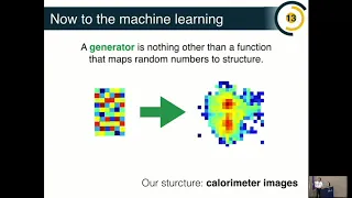
Okay. So now that's the physics background. Let me tell you about machine learning, so I think you've heard of it earlier about what a generator is, but in this context, I like to think of generators as a function that map's noise to structure. um So this is trans stands. Some random noise and I want to have a model that learns that to generate that into structure in our structure. Here is going to be calorimeter images, so we're going to think of a calorimeter as an image, and then we want to use generative model.

A

In this case, you can to generate those images, okay, so this is what a calorimeter calorimeter image might look like. So I have some chunk of material, that's segmented, so it's like a pixelated object and say we shoot some particles at it and those particles leave energy. Is that go through the segmented object and I can then think of this as a grayscale, a single, one-dimensional, grayscale image, where the pixel intensity that you see here corresponds to the energy deposited in that part of the detector. So this is great.

A

I now have an image grayscale image which I can use for generation now in practice. It's actually much more complicated in this, because we don't just have single images like this actually turns out that our detector has multiple layers. That's already a complication, but, more importantly, the segmentation on each layer is not the same. So imagine you have an RGB image where the red, green and blue channels all have different pixel sizes. So that's a significant challenge that we also would like to overcome with with these approaches.

A

Now, just to give you a sense, these images are roughly something like 30 by 30, so it wasn't dimensional, so the size of the problem, you're thinking of it as like a probability distribution is something like a thousand dimensional. Probably distribution and we'd like to generate three images in this particular example that have different granularities and have a causal structure. So clearly, the image for the third layer depends on the image for the second layer, okay, and so our strategy to attack this problem is with gans.

A

You heard a lot about games earlier and so I don't want to spend too much time introducing them, but just as a reminder again again has two components: a generator network and a discriminator network. So the generator network learns to Mountain oyster structure. That's what this one takes.

A

Noise map, strength images and then we have another one to discriminate or network that tells tries to distinguish between generated images and real images and in this cake, in this case, our real images are actually still synthetic, because the idea is trying to learn a simulator and make it faster. So we have images from a physics-based emulator, that's very slow, and then we have.

A

We learn a generative model to reproduce the simulator and the discriminator is just supposed to distinguish between the two and decide if it's looks realistic within the structure of the space simulator or not great. So the noise is a choice. It's a hyper parameter in this case. We we can pick a multi-dimensional Gaussian to start with, and this generator depends on what noise you pick.

A

So you start with some noise structure and the generator will learn to map into the into the structured images and if I use a different noise, it'll burn or different generator and they're, obviously related up to a Jacobian.

A

Okay, so now the model there's been a lot of information on this slide, so don't worry, I'm going to spend a few minutes on it. So this is the Callaghan. So it's again for doing color simulation, it's very fashionable to pend the word something in front of Gann, and so this is our catalog and and so basically, it has a structure where it takes as inputs a few things, so first the latent space.

A

So this is the noise, so in a thousand dimensional 18 space, but you can think of is just a very high dimensional multi-dimensional Gaussian in this case it's a thousand twenty-four dimensional, and then this whole structure here is that function that map's this noise into three images. So the output of one run of the generator is three images that correspond to each of the layers. Now we also have, as we want this neural network, to be able to be conditioned on various features, so in particular we want to be able to say what is the?

A

What do? The images look like, depending on the energy of the incoming particle, so we feed, in addition to the latent space, the energy of the incoming particle, and then we have basically three repeated units and these three repeated units are going to generate images for each of the layers and all the other structure here basically is to build in the causality between the layers.

A

So the first thing we do is we generate an image for the first layer and I'm going to tell you what this la GaN means in just a second, but for now it's a black box that generates an image of some size, and then we want to do.

A

Is we take that image and we resize it to be the same granularity as the second layer, and then we combine it with a totally independent, random, random image for the second layer using this structure here, and that gives us a new image which has some input from totally random input. This is independent and a contribution from the first layer so that it can know about the causal structure between the first layer, the second layer.

A

We then take the output of this combination and resize it once again to make it the same granularity as the last layer, and then this is combined with another independent random image from the that represents the third layer, and these two are once again combined to get an image which knows about the image in the previous layer, and so in this way we have three images all with some randomness, but also knowing something about the causality of the structure.

A

Oh, it definitely matters because the I think about the picture, so we're shooting particles from one direction. So they definitely come from this side and go to that side, and the granularities are also not the same, which makes it work.

A

Ok, so there few other bits I want to tell you about so for, like I said, we condition on energy, but we also want to present condition on particle type and particle type is a discrete is discrete so, whether it's like an electron or a proton, we found it was actually better to make different networks than to share I have the same network, but this I think is another hyper parameter that one could optimize and our images are also very sparse.

A

So, unlike images of celebrities where most of the pixels are activated, our images are very sparse and in fact many of the pixels are just totally zero, there's no energy deposited, and so for this reason it's useful. The vaccination functions like the relu, which help encourage sparsely okay. So this is the generator side, good right right right. So here it's a thousand dimensional yeah, it's exactly it's the same time as much related space. This is also a choice: oh and how it's divided up doesn't great question.

A

So there are many properties of this network which can be optimized and, in particular, the size, the latent space, the size and structure of the light in space. So we did not optimize it all the size or structure and we basically picked a thousand. That's a big number and roughly the size of the dimensionality of the problem lays if it's like roughly a thousand dimensional problems.

A

So we expect that something roughly a thousand should be good, but this is definitely area where one okay, so, in addition to the generator we have to have a disk or meter. So this is the the adversary to the generator Network and it looks very similar, but basically it's enough to run in the opposite direction. So this one takes as input three images and it produces classification so whether it's real or fake, and so as before, there are three there images one from each layer. They get fed into this block.

A

Once again, this black box block box, which black box block, which I will describe in just a second yeah, and so basically there. There are a couple of important features here. So one is that if we take a particle, that say has some amount of energy and we showed you, article emitter and it's totally absorbed in the calorimeter.

A

We want to make sure that the energy deposited on all the layers is equal to the energy of the initial particle, so that there's some kind of conservation of energy and in the in the generator structure, you see there's nothing that enforces that it could, in principle, generate energies for the three layers that are not conserving that don't--don't, some initial energy.

A

So what we want to do is we first build in some features so that we estimate the energy from each layer and then we're gonna feed the energy, the total energy reconstructed energy as a feature into this classifier start of enforce this energy conservation property. So it knows that it should be looking for. Kellerman are images that preserve that concert of energy. The other piece that we have is called mini bat discrimination, and the idea here is that if you look at single images, it's very hard to tell if it's real or fake.

A

But if you look at a small ensemble of images, it can be easier to tell because you can start estimating some statistical properties of your generated images, and so many bet discriminations that takes a mini batch, so a small set and from that computes features which can then be fed into a fully connected Network down the line to compute the full classifier that does the real versus fake, and so this neural network, which is the screaming of parties combined with a generator part and they fight it out until they, the discriminator, is totally confused and that's how it proceeded.

A

So now before I tell you how the results look like I have to tell you what this black boxes, so it so it's called la. So the la stands for locally aware, and in particular, this piece is composed of locally connected layers, and so I'd say what that means. So you've probably heard about convolutional neural networks and convolutional layers, so I'm adding you've an image.

A

The de-facto approach for image data is to use accomplish normal Network when you have some kind of filter and the filter is flipped across the image, and this gives us the output for a given filter, and you have many filters, and this is how we can take advantage of images that are trap. Translational invariance, because this this complement procedure here doesn't depend on where features are inside the image.

A

Now, the challenge with our art images is that we've already pre processed them, because we know where the direction of the particle was, and we know that should be the center of the image. And so, as a result, our images are not translationally invariant and so one can still use convolutional networks, but there's no translational invariance to advantage of, and so as a result. You want to do something a bit different now accomplished.

A

One will know which are still very powerful because of because of the weight sharing, they have far fewer parameters than a fully connected Network. So in these, in this case, for instance, the number of parameters of a CNN scales with the filter size and not with the image size. If you have a fully connected network, the number of parameter scales, commet Oracle E- with with the size of image number of pixels, whereas here it's basically fixed- you can have a much bigger image and have a fixed filter size that the number of parameters doesn't change.

A

So we try to have a compromise between a fully connected Network and a convolutional network, and the compromise is called a locally connected network and the idea is you take an image we divide it into patches and then in each patch. You have accomplished on network basically, so you have filters which are shared across different bits of the image. This is the still has some weight sharing, but it's not global weight sharing.

A

So imagine, I have my patches and then these I have a set of filters for each patch and then those so in these patches may be. The size of the filter sets the number of parameters. So this is nice because it takes advantage of the parameter reduction that we get from commercial networks, but it has more. Local structure can learn more easily. Local features that are not translationally, invariant, then accomplish will not work in can learn.

A

Okay, so let's see how it works in practice. So here are some images. The average images over many many examples for the physics-based we're trying to learn for the three different layers, and this is for the Gann and you can see you buy I. It seems to do pretty pretty well. So the z axis here is logarithmic. Lease is exponentially spaced. You can see that over many orders of magnitude, it's really getting the bulk structure correct.

A

This is a pretty weak test of the Gann, because these are just a few commercial images that are averaged but we'd like to know how well it's able to reproduce this multi thousand dimensional distribution.

A

Okay, so one thing we can do is we can take some features of the thousand Mitchell distribution and look at their histogram of those features. So, for instance, I can ask what is the distribution of the energy total energy in the first layer? So this is just like a sum over all the cells in the first layer and what's in the distribution of the energy, and so the filled in mr. Graham's. Here are the physics, bass, simulator and the other ones are the game, and so you see qualitatively over many orders of magnitude.

A

It does seem to reproduce some of the right features for different particles.

A

So these three lines are different particles, there's electrons, photons and then pi on, which is like a lighter version of the proton, but you, but there are some some quality of differences in a few places, so clearly there's room for improvement and we can repeat the same procedure for this middle layer and the third layer now as I know down here at the moment these features are not included in the training, but if there's any particular feature that you wanted to you is you can of course build it into the training.

A

Remember in the discriminator network we built in some energy conservation requirements, so we could always put in these these distributions as well I want to have at least some hold out in order to validate the procedure now. This brings me to one of the key challenges of gand training, which is that it's hard to validate a thousand eventual distribution, there's basically no good way at the moment for doing that. Quantitatively, so you could take some other some anyone, demential distribution, you like in this case it's the depth, weighted total energy.

A

So you take the total energy and weigh that by how far it is which which layer it's on, and you can look at this distribution just like the one from the last distribution- and you see qualitatively it looks okay, but how do I know it's doing well in the full thousand Mitchell distribution, with all the several correlations now in the industry? Usually you quality.

A

If you look at images- and you say, does this look like Angelina Jolie- and this is look, this looks like Brad Pitt and usually that's efficient, but in this case for scientific quality imprints on you know, theory and everything, that's an usually insufficient, and so this is I would say a big open research, question and I think that science applications have a lot to say about how we can quantify how well quantitatively, how well McCann is performing these tasks.

A

Okay, related is, you might want to ask questions about overtraining, so if you have more complicated because well, we still can't visualize it Michell space. We can. We can still ask some questions, so you might ask the question: is the neural network memorizing so that the cont'd, uh the analog of overtraining sort of generator, is just literally repeating to you the thing to give it during training?

A

That would be like memorizing and you might also be worried about another thing called mode claps, which I know is discussed earlier, which is if your generator is only generating a small subset of the full range of possibilities and they're very realistic, but they don't cover the full range of possibilities. um So that's called bode claps and one one you can sort of probe. That is to look at the distance, in some sense between your generated images and the real images and then between generated images and themselves.

A

So, for instance, in this case, these these plots show a histogram of the distance in Euclidean space I. Think of my thousand dimensional image is just a vector in Euclidean space, the the distance between a generated images generated image and the nearest physics image. This is take a take. A generated by earth take a generated, find the nearest physics. This is physics from the nearest generated and basically, if these were Delta functions at zero, what you would know it's memorizing, so they're not Delta functions at zero, that's good!

A

So it doesn't look like it's obviously memorizing the input and, for the most part, gans are really bad at memorizing. So this was not a surprise, but ganz do have a problem with mode collapse and another way to one way to probe mode collapse is to ask take an image and ask where the distribution of the distance with his nearest image. So this is began and all the nearest and neighbors- and this is the generator, the physics one and all the nearest physics neighbors.

A

So you would imagine if there was some region of the full set of possibilities. That's being over sampled, you would see a spike at zero. Basically, that would say that there's some region, that's being over sampled, so there's some images which are very close to other images in the sample and if you compare all four of these images, there's no obvious spike at zero and they look qualitatively the same as well. So the gamma images are basically just as far apart from the nearest kin image as they are from a physics image.

A

So it seems like it's interpreting pretty well, although if you stare very quantitatively these images, you see that, for instance, there are these spikes up here that are not down here. So this is a indication that there's no mode collapse that we're training, but but clearly this is only a one-dimensional projection of this. The high dimensional space, okay and the last thing I think want to mention about the results, is when extrapolating so ganzar a really good at interpolating.

A

So if you can go from Angelina Jolie to Brad Pitt, but they're, not so good at then extrapolating to someone else, but in our context we can ask the question what, if I query again to give me a particle whose energy it's never seen before and as long as there's no physical effects that happen for that energy between the energy trained and a new energy in principle, it should give something sensible.

A

So here you can see we queried for a particle whose energy was 150 in some units which and that the training stopped at 100, and actually the reconstructed energy is close to 150. So that's good. We read 100 150 and it basically still the energy conservation that was built into the network survived until 150. Now, there's a it's clearly, not not outsider 200. So these images look a bit different, but still it seems like they're there they're able to learn something a bit outside of the domain that they were trained on.

A

Okay, so so far, I've basically been talking about images where we have fixed energy and sampling the input, leighton spann. Imagine doing the opposite. You can imagine, fixing the energy and varying the latent space to see how the neural network has learned the dependence on the latent space and if they have any physical meeting, so in particular what we can do is we can condition condition on the latent variables and see how the shower changes. So one thing we can do is we can say this is a. This is a for a fixed particle.

A

We don't change the latent space, we fixed the noise and we just vary the energy and you can ask: how do the images look like if we vary the energy but fix the noise? And basically, as you increase the energy, the particles are becoming deeper inside the calorimeter, which makes sense, so it's a little hard to see that. But basically this is the energy in the zeroth layer.

A

The first layer in the second layer and the amount of energy on each layer is increasing, which is good, because there's more energy overall and especially the last layer, has quite a significant amount, more energy, because the particles are making it deeper into this into this calorimeter, and we can also do things like move the position of the particle, and so here you can see the particle moves as we image moves as we change the input position, and so this allows us to sort of probe that the neural network is doing the right thing and also is sort of a nice feature that we have built into the structure of the gann.

A

Okay and then the whole point of this procedure. This process, I told you was to speed up the physics-based emulator. So here just some timing results. We have our slow physics based emulator takes a long time to generate an image and for these single particle images. You know in this benchmark computer. It took something like thousand milliseconds and if you do, you use batching on GPU with again it's much much faster. It can be like five orders of magnitude faster, which is also surprising cuz.

A

It's not doing all the physics, the deep physics that the physics basically are doing, and so this is one of the promising aspects of this approach, and very last thing. I want to say before I finish is that everything I've shown you so far is sort of in the context of a small study using standalone synthetic data.

A

But of course, ultimately, we would like to integrate this workflow into one of the big Large Hadron Collider collaborations, and this is a challenge in and of itself, because we have many thousands of collaborators, a very large extensive and old software code base, but so far we're managing- and here is a plot which I think is really nice. It's actually a random plot, but it shows that there's again so I like what this plot is.

A

Two things there's the word Gann and the word Atlas basically shows that in a big LHC collaboration, we've managed to integrate again and actually also a variational, auto encoder into the software stack to do some 2d comparisons and the actual distributions here are not quite so relevant because it's still early days, okay. So that brings me to the end of my presentation, so neural network generation, I think, is a systematic, the improvable path forward to increase the fidelity, and hopefully the speed of surrogate models.

A

Employing these tools is really a challenge and I think there's a lot of interesting technical as well as machine learning and scientific challenges ahead of us in particular. The key challenge, which is trying to identify win again, is a good gun and then identifying when we do know that we're training when we when we can stop and then compare to the state of the art I'd like to thing my my collaborators on various projects and I slay, the slides I, think, should be online and you're and you're.

A

Welcome to it to look at all the references, including a code in and synthetic data, and that range to the end.

A